Fully Coupled Thermal Structural Analysis With Abaqus

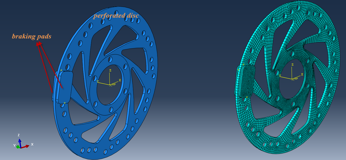
In this post, we will be showing some of the capabilities of Abaqus for performing fully coupled thermal-structural analyses. In particular, an exemplary geometry of a mountain bike's perforated disc together with the breaking pads (included in the caliper-not modelled) will be used to show some of Abaqus' conjugate heat transfer and multiphysics capabilities.

The geometry and mesh of the full assembly can be seen in Figure 1.

Figure 1: Discbrake assembly and mesh discretization.

Analysis Procedures

First, the disc will be rotated, in order to acquire a steady state rotational velocity, comparable to cycling. Abaqus standard will be used for this procedure. in particular, a steady state coupled temperature-displacement analysis step will be performed. Restart output will be requested.

This will allow for the importing of the steady state implicit analysis results, into Abaqus Explicit. Those results will be used as an initial state for the transient coupled temperature-displacement analysis step that will be performed. During that step the rotating disc will be decellerated to a halt.

Steady State Coupled Analysis (Abaqus Standard)

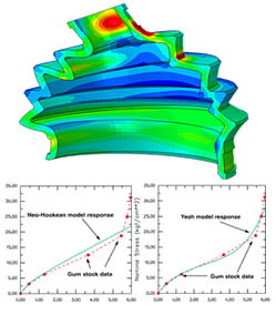
Since the thermal domain is of significant importance for this investigation, heat dissipation will be modelled. There is therefore the need to assign respectful temperature dependent material properties for both the perforated disc as well as for the braking pads. This can be done as usual, from the property module in Abaqus. A detail from the respectful properties of the braking pads' composite material is given in Figure 2.

Figure 2: Temperature dependant thermal properties of composite braking pads.

Thermal Loads

Convection and radiation to the ambient temperature (sink) of 20 degrees Celsius, will occur on the surfaces of the disc. 

In order to model this types of conjugate heat transfer, it is necessary to define a film condition and a radiation condition for convection and radiation respectively. 

This can be done via the Interaction module.

A relevant detail is given in Figure 3.

Figure 3: Convection and Radiation Interactions for the disc.

Since a radiation condition is modelled here, this necessitates defining the absolute zero temperature and the Stefan-Boltzmann constant. You can enter their values by editing the Model's attributes.

Initial Temperature

Since we have modelled convection and radiation for the rotating disc, we also need to establish an ambient temperature of 20 degrees Celsius. This can be done normally via the predefined field for this analysis.

Loads and Boundary Conditions

In terms of loading, we only need to apply a rotational velocity of 250 rad/sec on the disc. We can do this by applying a rotational body force on the disc. The magnitude should be 250 rad/sec and the vector should match the Y-axis (Y-axis rotation).

In terms of boundary conditions, we need to constrain the reference point at the center of the disc at an initial step. Then for the steady state rotation step, we can release the respectful rotational degree of freedom (in this example it is UR2).

To model equivalent boundary conditions on the disc, in order to match its connection to the the axle of the bicycle that is not explicitly modelled, we need to constrain the portion of the disc that is bolted to the bicycle and create an MPC to mimic a pin connection ,as it is demonstrated in Figure 4.

Figure 4: Steady State boundary Conditions for the perforated disc.

Then we can create and submit the corresponding job. A detail from the results of the Steady state analysis in Standard, is given in Figure 5 below.

Figure 5:Von Mises stresses (MPa) and Nodal Temperatures (degs Celsius) at the end of the Steady State coupled analysis in Standard.

Transient Coupled Analysis (Abaqus Explicit)

As was previously mentioned, the preceeding steady state analysis, will be imported into Abaqus Explicit in order to continue with decelerating the rotating disc to a halt, by applying pressure on it via the braking pads.

The actual details/conventions of the process of importing the steady state analysis into Abaqus Explicit will not be covered here. Attention should be given on the following:

-surfaces and sets referring to the import analysis should also be present in the transient model (explicit). Of course new sets and surfaces can be defined in the transient model.

-an balancing/equilibrium step between the steady state and transient analysis should be included in order to balance the dynamic results upon importing them. This balancing step should have all loads and BCs from the steady state step propagated, to maintain consistency.

Thermal Loads

The pre-existing convection and radiation of the perforated disc, should be sustained for the transient step in Explicit. Additionaly for this step, since heat dissipation will take place also along the interface between the composite pads interacting with the disc during braking, an additional contact interaction (General contact) with appropriate thermal properties should be created. 

Thermal Interface

Frictional heat will be generated under the braking action  between disc and pads but also the effect of gap conductance will be included. A relevant interaction property was therefore defined. A detail of that  property is given in Figure 6.

Figure 6: Thermal interface properties for the composite pads.

Initial Temperature

As for the preceeding analysis, an initial sink temperature should be present for the perforated disc. Additionally for the transient step, the same initial temperature will need to be defined for the composite brake pads to match the initial temperature of the domain. This can be done again via the predefined field for this analysis.

Loads and Boundary Conditions 

A pressure load acting on the pads should be assigned for the braking step. Also the displacement of the braking pads should be constrained in certain axes. Both of those details, are depicted in Figure 7. The pad faces upon which the boundary conditions are imposed (in order to limit the pad motion on the Y-axis), should also be used to apply pressure loads for braking down the disc. For this example, a pressure load of  3.5 MPa per braking pad was applied. A relevant detail on the constrained pad faces is given below.

Figure 7: Boundary conditions, limiting the lateral motion of the braking pads.

Last but not least, with respect to the rotating disc, remember to release the disc's rotational velocity for the braking step (VR2 should be ticked of) in order to achieve the full braking down to a halt.

With respect to the time period for the transient step, for the first run this is merely an estimate, an educated guess.  A relevant video of von Mises stress (MPa) and nodal temperatures (degrees Celsius) is shown below.