In this blog I thought we could do a small dive into hyper and viscoelastic materials and how to model these in Abaqus. Many elastomers, rubbers and biological soft tissues exhibit such behaviours.
Introduction
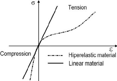
Hyperelastic materials, are materials that respond elastically even when they are subjected to large deformations. They have a highly non-linear stress-strain relation and are nearly incompressible (the shape may change, but overall volume is constant).

Figure 1. Example of hyperelastic material response compared to a linear elastic material (i.e. metal).
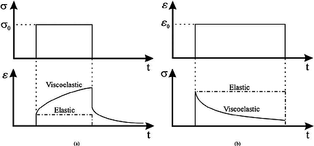
Viscoelastic materials, one the other hand, exhibit both viscous and elastic characteristics when undergoing deformation. Some polymers, wood and in particular human tissue have a viscoelastic response. For instance, creep (Figure 2 - left) means that under a constant stress (force), the strain (deformation) in the material will increase with time. Similarly, stress-relaxation (Figure 2 - right) means that if the strain (deformation) is kept constant, the stress (force) response will decrease in time.

Figure 2. Viscoelastic material response. (Left) Creep; (Right) Stress-relaxation.
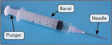
These two material responses can be model using Abaqus. So let's look at how to do this by considering an example. A typical syringe has three main components: the plunger, the barrel and the needle (Figure 3). One end of the plunger is capped with a rubber seal. So, how would we model this rubber cap if the material had hyper- and viscoelastic material properties.

Figure 3. Parts of a typical syringe.
FE Model Setup
Geometry and Mesh
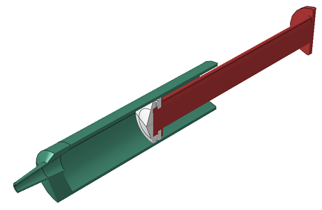
GrabCad has a nice syringe CAD model in Solidworks. After some defeaturing, the geometry was imported in Abaqus. We have the plunger (red), rubber (white) and the barrel (red). In this example we used a hex mesh for all instances and chose the mesh density so that the results are obtained in reasonable amount of time, while still being dense enough to make the results sensible. C3D8RH element were used. Hybrid elements are needed when modelling incompressible (v=0.5) or nearly incompressible (v=0.475) material behavior.

Figure 4. Syringe geometry imported from Solidworks.
Material Properties
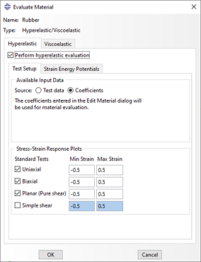
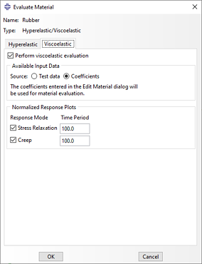
In terms of material properties, the plunger and barrel were a generic polypropylene, with isotropic elastic material properties from SolidWorks database. The rubber was modelled as a hyper- viscoelastic material. Abaqus has a two main options for considering this: 1) directly specifying the coefficients, in case the response can taken from literature, and 2) we can use test data and Abaqus will evaluate which material model best matches the test data (Figure 5). Please check our previous blog for more details here.


Figure 5. Material evaluation options in Abaqus.
In this case, we had coefficients from a previous workshop. The rubber end was modelled as a neo-hookean material (C10=200, d1=0), with the viscoelastic behavior specified using a Prony series.

Figure 6. Prony series coefficients.
Interactions
First we defined a general contact with a Friction coefficient of 0.8 and "hard" pressure-overclosure. The general contact algorithm resolves initial overclosures using strain-free adjustments by defaults. In this example, it is more sensible to treat initial overclosures as interference fits, assuming the rubber end is tightly fitted into the tube.
Steps, Loads and Boundary Conditions
The analysis was carried out in 3 steps:
- A static general step called "Step 1 - Interference fit" was defined with a duration of 1e-6 and an initial increment size 1e-7. In this step, we only resolve the initial interference fit.
- A static general step "Step 2- Compression" was defined. The duration and increment size was the same as in 1. Here, we Encastered the left part of the syringe tube. We defined a reference point and coupled it to the end of the plunger. We applied a displacement to this point. An overview of this is shown below.
- A visco procedure, "Step 3- Relaxation", was created. The time period was 50s and initial increment size was 0.1. The viscoelastic strain error rate tolerance was also 0.1. This step will calculate the stress relaxation of the rubber in 50s.
The very small step size in 1 and 2 are required since the visco procedure uses total time (not step time) to calculate time-dependent material properties. Additionally, the viscoelastic material properties are only considered in Visco, Coupled temp-disp and Dynamic procedures. Default History and Field Output requests were used.

Figure 7. Boundary conditions and interactions.
Results
Interference Fit
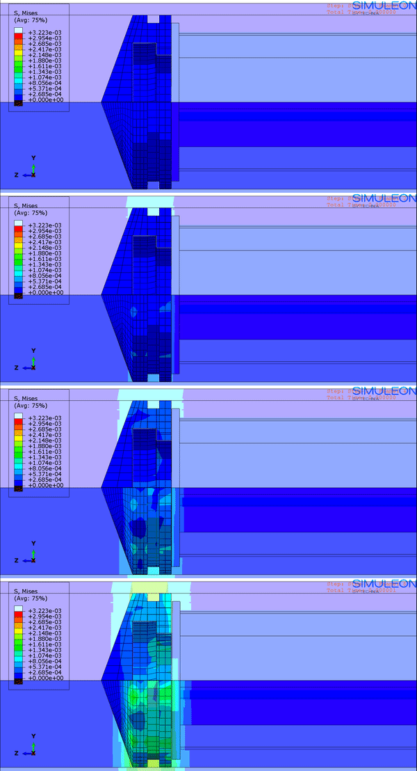
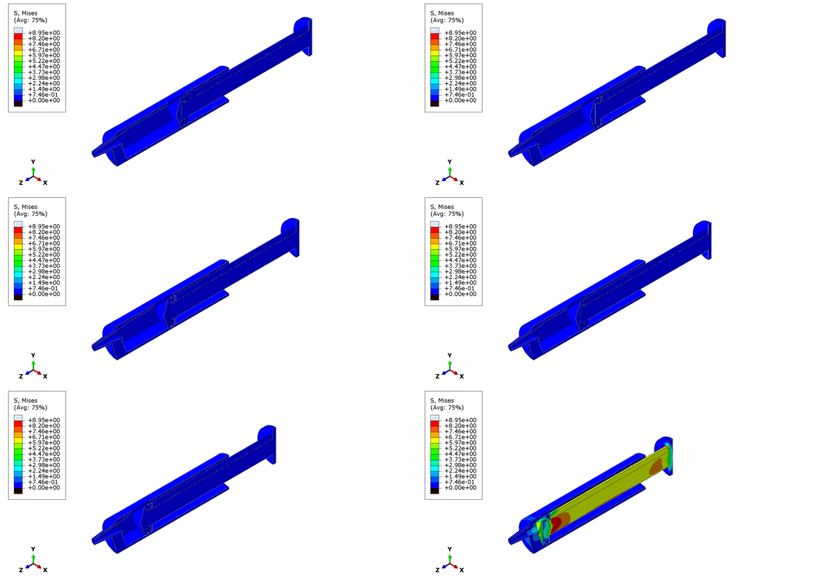
In this step, the initial overclosures between the rubber and the plunger and between the rubber and the barrel are gradually removed (Figure 8)

Figure 8. Interference fit animation.
Compression
The animation in Figure 8 shows the plunger and rubber displacement. Note that only at the end of the step the stresses become apparent on both the plunger itself and the rubber.

Figure 9. Compression animation.
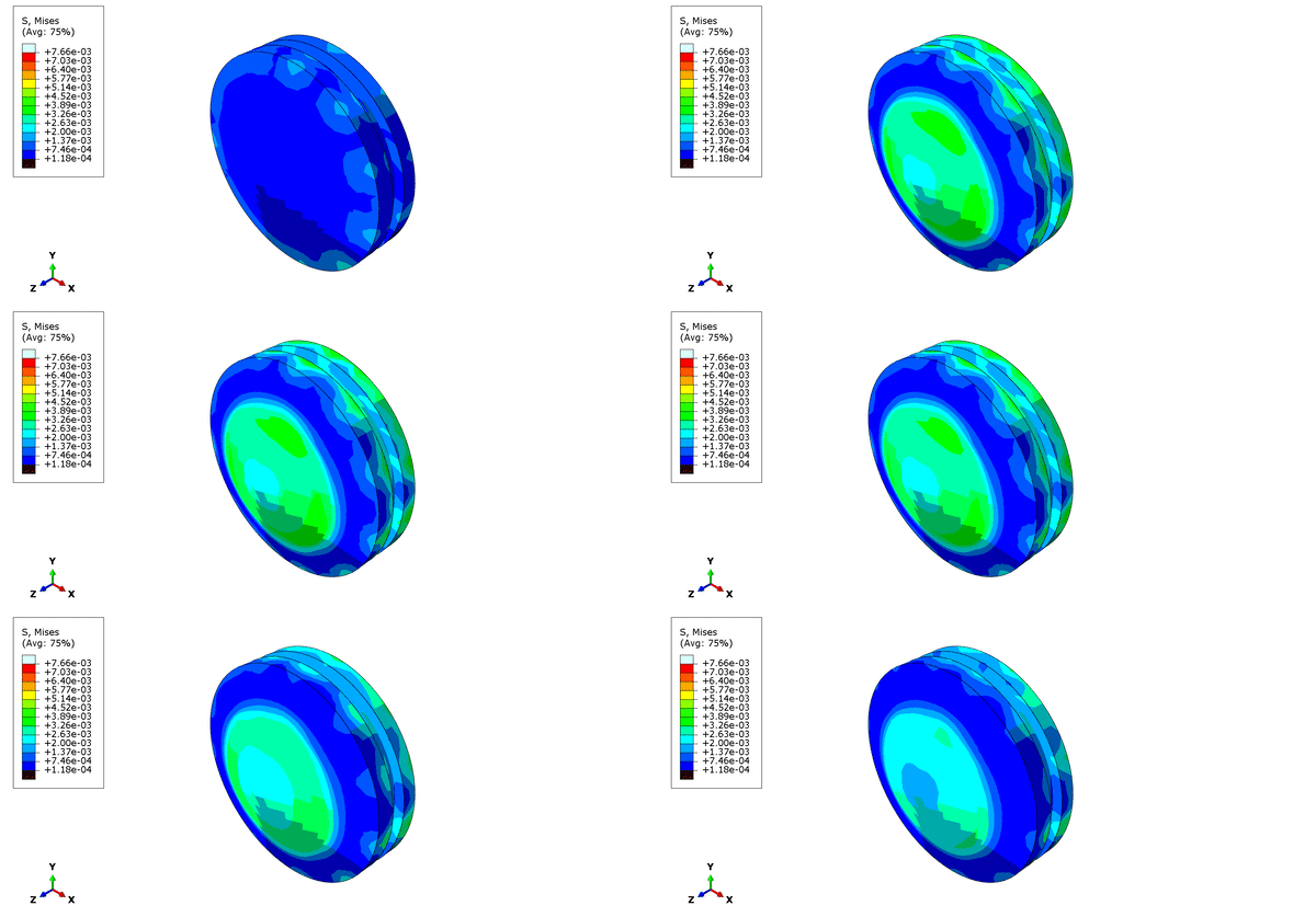
However, during the entire step, there are some small stresses on the rubber end as a result of the friction between it and the syringe barrel. These become apparent if the last frame is excluded from the animation.

Figure 10. Compression animation on rubber end, with the final frame.
Stress-Relaxation
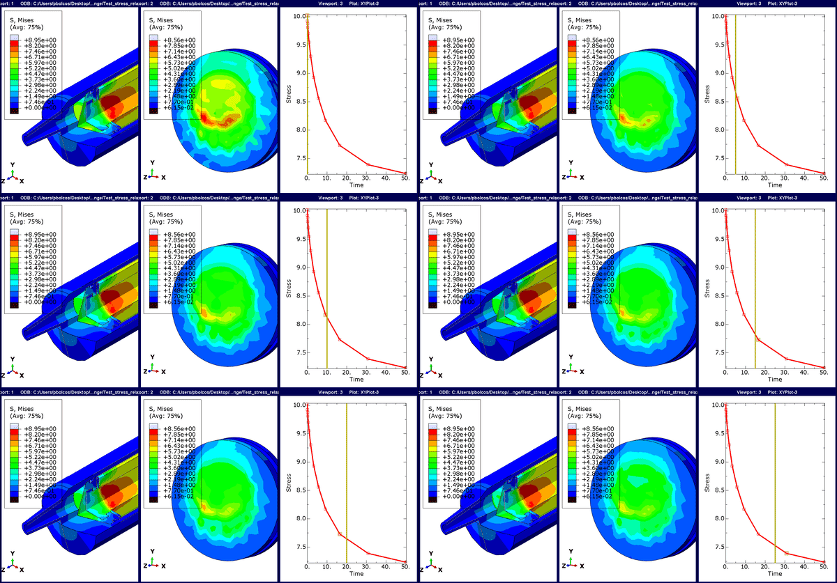
In this step, we can gradually see a reduction in the peak stresses due to viscoelastic effects.

Figure 11. Animation for stress-relaxation. The time history is time-based rather than the default frame-based option.
Discussion
We've shown how to consider hyper- and viscoelastic materials in Abaqus and what their effect is. There are a few things that need some further discussion.
Some may be wondering why consider the interference fit in an additional step and not combine it with the compression. Typically, the interference fit is resolved in the first increment by default. However, in some cases this may not be possible and the analysis may fail or have very large cutbacks. If a separate step is used, then these overclosures may be gradually resolved over multiple increments.
Unfortunately, hyper and viscoelastic properties for specific materials are not easily obtainable from web sources (i.e. MatWeb) and testing is required. The hyperelastic material, the quality of the results depends on the test data provided, so it is imperative to obtain experimental test data from multiple tests, such as: uniaxial, equibiaxial, planar and volumetric test. If the component is loaded mainly in compression, it is important that the test data has compressive loading, rather than tensile. Finally, the automatic evaluation of the material models gives some stability limit information, that should not be exceeded. A similar case could be made for the viscoelastic material properties derived from test data.


