Kinematic Vs Distributed Coupling Constraints in Abaqus

In this blog post, we will be discussing the differences between the kinematic and distributing constraints in Abaqus. The differences between these types of constraints will be highlighted in an example model.

Introduction and Usage

Surfaced based coupling constraints are used in Abaqus for the following purposes:

• To couple the motion of a collection of (slave) nodes on a surface to the motion of the reference node
• is of type=kinematic when the collection of nodes are to be coupled to the rigid body motion defined by the reference node.
• is of type=distributing when the collection of nodes are to be coupled to the rigid body motion defined by the reference node, in an average sense, by allowing control over the transmission of forces through weight factors specified at the coupling nodesIn terms of typical applications wherein the coupling constraints can be deployed, those are:
  • To apply loads or boundary conditions to a model. 
  • To distribute loads in a model, where the load distribution can be described with a moment-of-inertia expression.
  • To apply dimensionality transitions between continuum and structural (beam or truss) elements.
  • To model interactions with other constraints, such as connector elements. 

Coupling Constraint Definition

Coupling constraints in Abaqus are set up through the interaction module. The respective windows for setting up the coupling constraint in Abaqus, are shown in Figure 1 below.

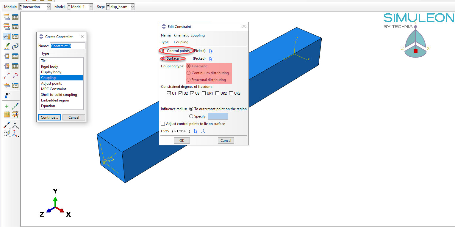
Figure 1: Windows in Abaqus  CAE for setting up kinematic/distributing coupling constraints.

What needs to be specified for a coupling constraint, is the reference node (or constraint control point), the coupling nodes, and the constraint type. The coupling constraint will then associate the reference node with the coupling nodes.

Kinematic Coupling Constraint

Kinematic coupling constrains the motion of the coupling nodes to the rigid body motion of the reference node. Kinematic constraints are imposed by eliminating the degrees of freedom at the coupling nodes. This means that once the user constrains any combination of displacement degrees of freedom at a coupling node, additional displacement constraints, BCs, MPCs, etc. cannot be applied further to that coupling nodes. This limitation is also present , when rotational degrees of freedom have been constrained at a coupling node (similarly to displacements).

The main modelling window of the kinematic constraint, is shown in Figure 2, below.

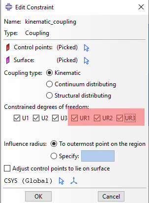
Figure 2: Kinematic coupling constraint window and available degrees of freedom.

When, in a kinematic constraint, all 3 translational DOFs are constrained, the coupling nodes will follow the rigid body motion of the reference node.

Constraining, different combinations of rotational degrees of freedom (UR) , will result in rotational behavior in the coupling nodes, that will be identical to existing MPCs(Multi Point Constaints) in Abaqus. In specific:

• If all 3 rotational DOFs are selected (along with the 3 translational DOFs) , then the kinematic coupling is equivalent to MPC Beam.
• If 2 rotational DOFs are selected, the kinematic coupling is equivalent to MPC Revolute in Abaqus Standard.
• If 1 rotational DOFs is selected, the kinematic coupling is equivalent to MPC UNIVERSAL in Abaqus Standard.

Distributing Coupling Constraint

Distributing coupling constrains the motion of the coupling nodes to the translation and rotation of the reference node. This constraint, unlike the kinematic one, is enforced in an average sense in a way that enables the control of the transmission loads, from the reference node, to the coupling ones, by using weight factors at the coupling nodes. The main modelling window of the kinematic constraint, is shown in Figure 3, below.

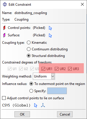
Figure 3: Distributing coupling constraint window and available degrees of freedom

In a 3 dimensional analysis, the user can release all three moment constraints(UR1-UR3), by specifying only translational degrees of freedom in the constraint. In such a case, only translational degrees of freedom are active in the reference node. The influence on the behavior of the constrained nodes in this case, will be demonstrated in the Abaqus example shown later in this post.

Example Model 

Geometry and Mesh

The exemplary geometry is shown meshed in Figure 4. It is a beam, modelled with 3d solid continuum elements (C3D8I). Its cross section is rectangular (250x250 mm) and its length is equal to 2m.

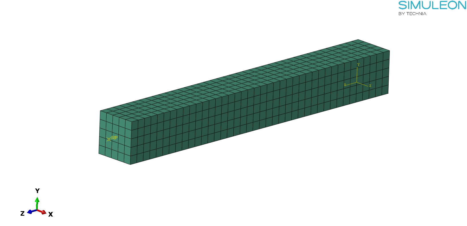
Figure 4: Meshed geometry of the example

Loads and BCs

The beam is fully fixed on its right end, while a vertical displacement (-Y) is applied on a remote point (RP), 50 mm away from the beams left end.  Appropriate BCs were imposed on the remote point(also the reference node for the coupling), to constrain lateral(X) and axial (Z) displacement. Those are shown, in Figure 5.

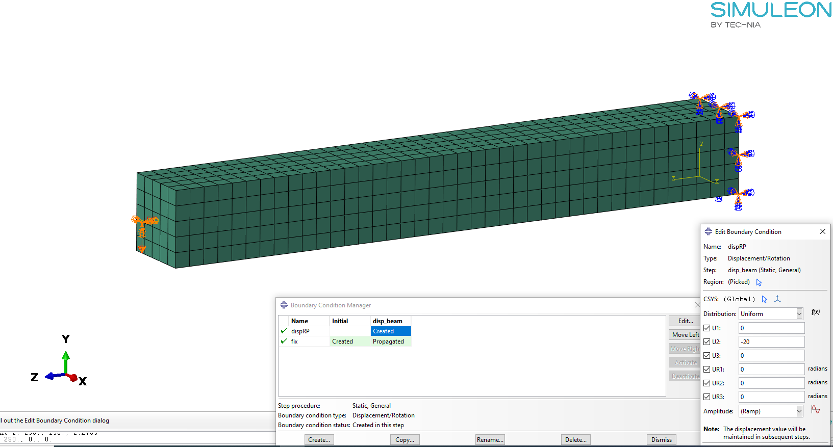
Figure 5: Loads and BCs of the example

The remote point is coupled to the left end face of the beam, using both a kinematic coupling, as well as a distributing coupling, for results comparison. The settings used for the run with the kinematic constraints are shown, in Figure 6.  Also the setting modification for implementing the distributing coupling constraint, is shown in the red box in Figure 6. All Dofs of the coupling nodes are constrained to those of the reference node, for both types of couplings.

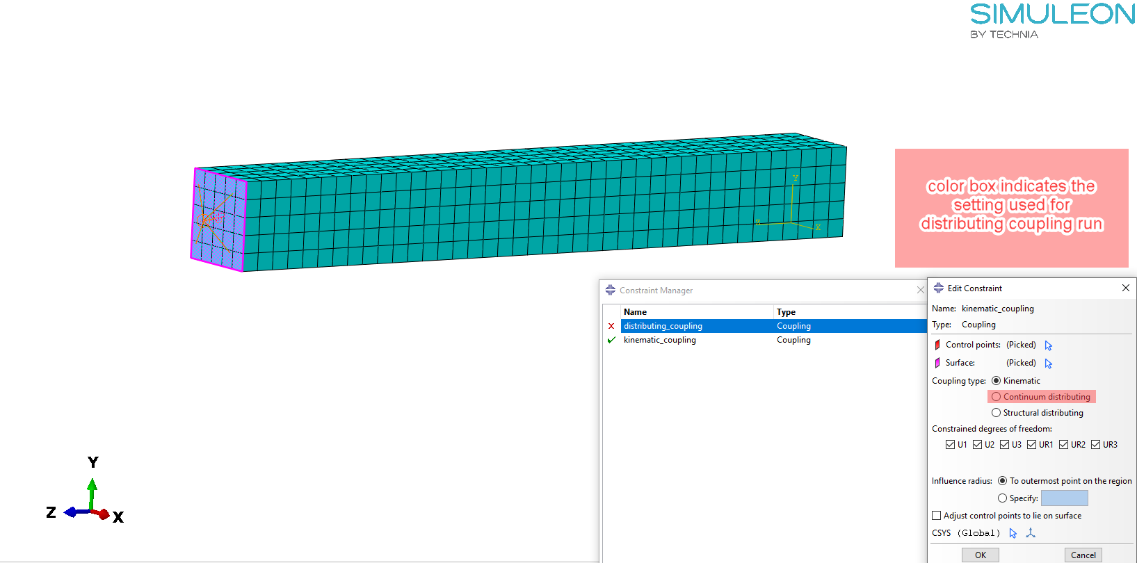
Figure 6: Coupling constraint definitions

Material 

As a material law, a linear elastic one was implemented for the example, utilizing generic steel properties for the Young's modulus and Poisson's ratio.

Results Comparison

The deformed shape of the beam, loaded under vertical displacement (20mm), is shown (exagerrated 20 times) in Figure 7. This is superimposed against the undeformed shape(grey color) and the deflected shape is quite comparable between the two coupling constraints (kinematic vs distributing).

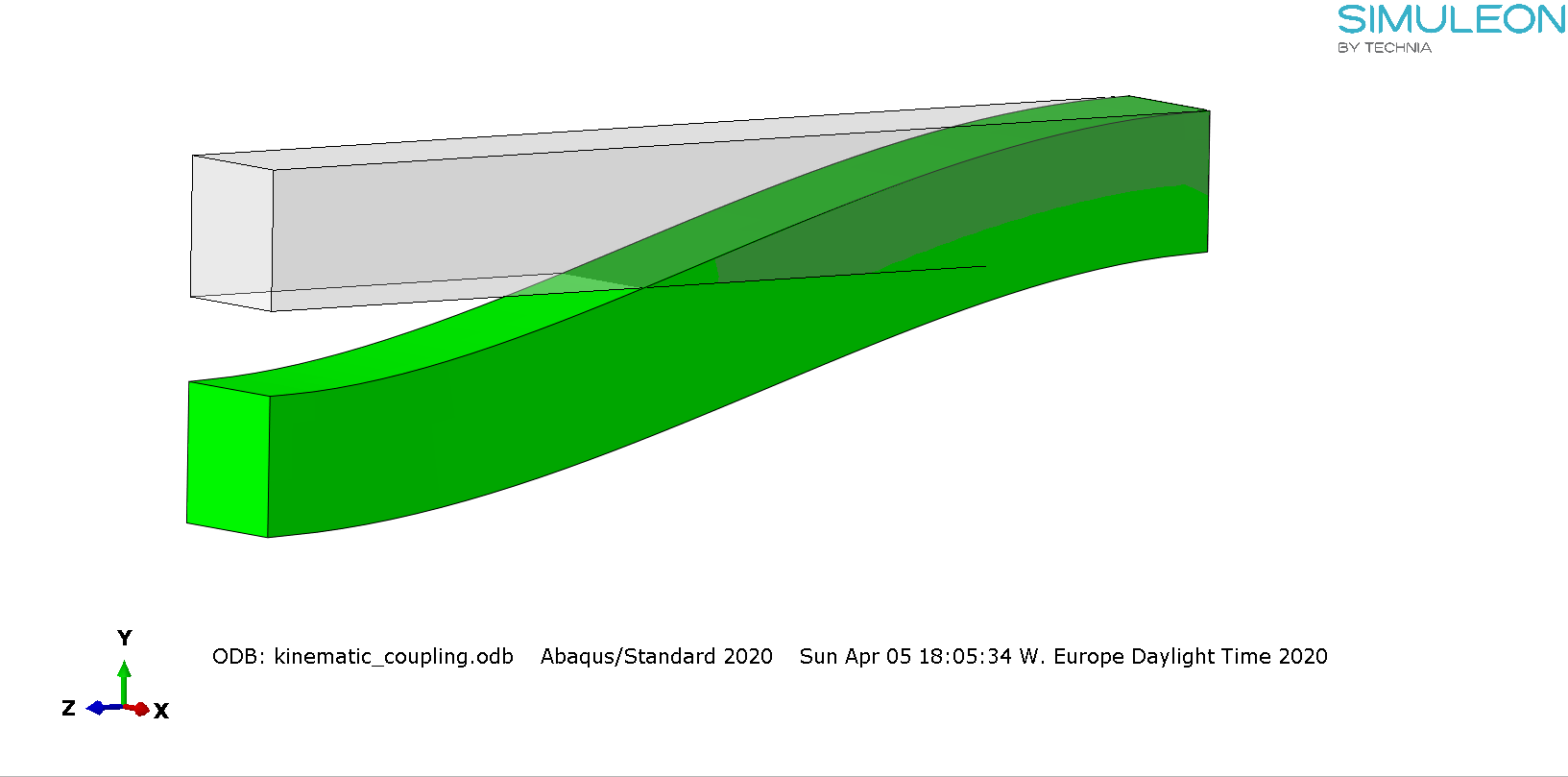
Figure 7: Deformed vs undeformed shape  for the beam of the example

A closer look at the contour plots of axial displacement (Z) , can reveal the differences in between the two coupling constraints. This detail is given in Figure 8 where U3 displacements are shown. The contour limits have been adjusted accordingly, to enhance showing results in the left end face of the beam, that contained the coupling nodes. The upper contour plot is from the kinematic coupling run, and the lower one, from the distributing coupling run.

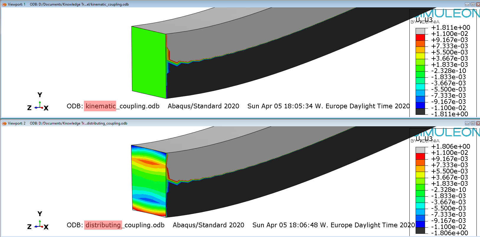
Figure 8: U3 displacement comparison (in mm)

For the kinematic constraint (upper plot) , all DOFs of the coupling nodes are coupled to the rigid body motion nodes of the reference nodes. Therefore the U3 displacement of those nodes is strictly zero, obeying the boundary conditions applied on the reference node. Essentially in a kinematic coupling, all constrained DOFs on the coupling nodes, are eliminated.

The distributing constraint (lower plot) , on the other hand, allows for relative deformation of the coupling nodes, as can be seen on the plot (red and blue regions with non zero U3 displacement).

Results Comparison 2

As an additional investigation, the constrained DOFs of both coupling types were modified and the analyses were rerun. This was done, to investigate the differences in constraint enforcement between kinematic and distributing couplings, and to also understand how the distributing coupling is imposed.

After the modification, only the translational degrees of freedom (U1,U2,U3), were coupled in  coupling definitions. The rest of the model input, remained the same.

A side view of the  deformed shapes from both runs, against the undeformed ones, are shown in Figure 9.

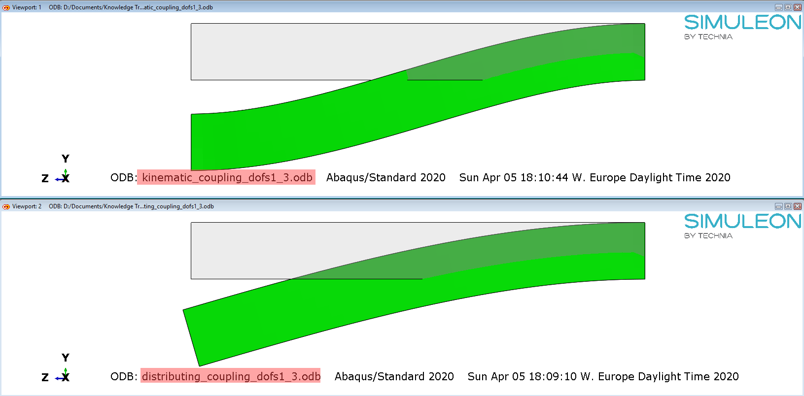
Figure 9: deformed shapes with URs  released in the coupling definitions.

It can be seen from the lower plot, that the beam's end is allowed to rotate, when using a distributing coupling. This happens, because the rotational degrees of freedom on the reference node (RP-all URs were constained in the model input), are active, only when at least one rotational degree of freedom of the coupling nodes is coupled. If not (which is the case here), the URs of the refernce node remain inactive, allowing the beam's end to rotate. This is not the case with the kinematic coupling.

Final Remarks

• A kinematic coupling is useful, when a particular kinematic mode of a structure must be suppressed. An application can be for example, the pure bending of thin, shell like structures, wherein the cross section must ovalize but remain plane.
• A distributing coupling allows more control over the distribution of the load from the RP to the coupled nodes. Other options (than "uniform") are available. This is not possible with the kinematic coupling.
• A continuum coupling is a special type of coupling, that essentially only allows the transfer of forces (and not moments) in the coupling nodes. This has application specific benefits. More information can be found here.
• A distributing coupling must always constrain all available translational degrees of freedom at the coupling nodes. This is not the case for the kinematic coupling.
• Once at least one (or a combination) degree of freedom has been coupled in the coupling nodes of a kinematic coupling, all DOFs are eliminated. This is not the case with a distributing coupling.