In this blog post, we will be discussing about steel fibre reinforced concrete (termed as SFRC) and will be showcasing a way (more modelling ways do exist)  to model the interaction between the steel fibre (reinforcement) and the concrete (matrix).

Introduction

Plain concrete is a widely used engineering material. When it deforms under compressive loads, it exhibits a nonlinear behavior with high compressive strength. When loaded in tension however, concrete is weak and has a limited tensile strength, forming cracks that consequently induce a brittle unwanted type of failure. Engineering practices have tried to change that behavior, by deploying rebars, which are steel rods embedded in concrete. Additionally, SFRC has been developed. This type of concrete included discontinuous small steel fibers instead of distinct rebard inside its volume.

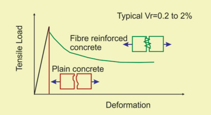
The reasoning behind both rebars in plain concrete and SFRC, is that the brittle tensile behavior that plain concrete exhibits, is  turned into a more ductile type of response as is depicted in Figure 1.

Figure 1: Concrete's behavior under tension

What happens is that when concrete cracks under tension, the rebars or SFs will undertake the tensile load, leading to this ductile response that is more preferable.

Fibre-Matrix Interface

In order for this to happen in the fea world, accurate modelling of the fibre-concrete interface is necessary. A graphical 2d representation of the interface, together with relevant terminology is shown in Figure 2.

Figure 1:Fibre-matrix interface

The interface is represented by the red lines in Figure 2.

The behavior of SFRC will be investigated via a pull out test of a fiber from the concrete. The pull out force and the failure mechanism relating to a pull out test of the steel fibre, is dependent on three distinct behaviors, that should be present at the fibre-concrete interface.

Adhesive bonding, debonding and frictional behavior. 

Adhesive Bonding

During the first stage of the fibre pull out, the response is governed by adhesion, existing between concrete and fibre. This bonding between the two materials, is due to the manufacturing method of the composite. Shear(traction) stresses are transferred to the concrete from the steel fibre via the interface. This requires the definition of a bond-slip relationship.

Debonding

While we continue to pull the fibre out, the shear stress present in the bond between fibre and concrete , continues to increase. At a certain maximum shear stress, the adhesive bonding of fibre-concrete, will start to fail. This will happen progressively and not instantaneously. Stresses are transferred normally, until the maximum stress is reached. This is the moment of the initiation of debonding. Past this point, decreased stresses will be transferred via the interface as debonding will have commenced. As the debonding evolves, lower stresses are transferred via the interface, until the interface fails (and the debonding is complete).

In order to model debonding, usually a traction separation law is required. This law needs to consider the following aspects. It needs to have a damage initiation defined( a maximum shear stress), as well as a damage evolution (a mathematical description of the progress of debonding). Last but not least, large displacements need to be accounted for, since debonding will induce them in the fe model.

Frictional Behavior

When the damage initiation relating to debonding has been reached, the frictional behavior comes into play.

As we continue to pull the steel fibre out of the concrete at this stage, the stresses generated at the fibre- matrix interface, will be the product of both friction and the damage evolution (progress of debonding). Stresses due to friction will still play their role, till the steel fibre is pulled out entirely from the concrete.

In order to include the frictional behavior in the common interface, we can use Coulomb friction. This frictional model, considers the shear stress occurring between two surfaces, as a fraction (=friction coefficient μ) of the normal stress acting on the surfaces. 

Abaqus modelling

The information provided above, will be showcased with an example in Abaqus. This will concern a pull out test of a steel fibre. An axisymmetric model will be used for this purpose.

Abaqus provides surface based contact pairs, that can be used to incorporate the three behaviors mentioned above while accurately considering large displacements. 

All we need to create, is contact pairs, between steel fibre and concrete, corresponding to their common interface, as shown in Figure 3 (based on the blog’s example).

Figure 3: Contact pair surfaces for blog's example 

The bond slip relationship, used for modelling adhesive bonding at the interface, is shown below. This is defined via the interaction property module of Abaqus. The values indicated in Figure 4 are exemplary.

Figure 4: Adhesive bonding interaction property

Figure 5, shows an exemplary debonding property relating to the damage initiation for the debonding stage.

Figure 5: Debonding initiation interaction property

Figure 6, shows an exemplary debonding property relating to the damage evolution for the debonding stage.

Figure 6: Debonding evolution interaction property

Lastly, figure 7, indicates an exemplary frictional interaction property, where Coulomb’s frictional model is used.

Figure 7: Frictional behavior  interaction property

It should be noted that for the selected frictional model, there needs to be a normal stress present at the common interface. If not, there is no shear stress active. In order to have a normal stress acting on the interface, two methods are commonly used. A shrinkage can be assigned for the concrete (predefined field+ thermal expansion coefficient). This will effectively create a compressive (normal) stress acting on the fibre-matrix interface which will activate Coulomb friction. This approach will be demonstrated with an axisymmetric example problem in this post. The loads and BCs can be seen in Figure 8.

Figure 8: Loads and BCs of blog's example

Alternatively , the straight steel fibre, can be pulled out , with a displacement, having  a vertical as well as a horizontal component. The magnitude of the horizontal component will be significantly lower than the vertical one, and it will serve the purpose of activating the frictional model. Additionally, the introduction of the horizontal “force” component, is a nice approach for investigating the influence of manufacturing imperfections. For example, a steel fiber might not be fully straight in reality (although intended), and as its pulled out, different frictional forces will be introduced at the common interface (less uniform) compared to the pull out of a fully straight steel fiber.

For this example, linear elastic material properties are used for both concrete and steel. At a future blog post, damage will be included for the concrete, with the use of the Concrete Damage Plasticity model. 

Results

Figure 9, shows the deformed geometry as well as the resulting normal stresses acting on the fibre-matrix interface, due to the shrinkage of the concrete. Remember than in order to be able to use Coulomb friction, we need to have normal stresses generated at the interface.

Figure 9: Stresses-deformation after shrinkage

Figure 10 shows the resulting normal stresses at the composite, after a pull out displacement of 3mm has been imposed on the top of the fibre.

Figure 10: Normal stresses at end of pull out

Figure 11, shows the resulting pull out force (RF2)  vs time and vs displacement. Past the peak of the curve (approx 90N) , both the debonding and the frictional models are active at the steel-fibre interface.

Figure 11: Pull out force (RF2 at top of fibre)

References

1. Biaxial stresses in steel fibre reinforced concrete: modelling the pull out-behaviour of a single steel fibre using FEM (master student thesis: an der Aa, P. J., 28 Feb 2014, TU/E- Department of built environment)