Modelling Hyperelastic Behavior Using Test Data in Abaqus

In this blog, the hyperelastic behaviour modelling in Abaqus will be discussed.  This will be implemented by fitting relevant experimental data with appropriate strain potential energy functions that are built-in in Abaqus and deciding on the function that best models the rubber materials behaviour. Additionally a finite element model will be demonstrated, wherein the designated material behaviour will be show cased.

Last but not least, in the process of explaining relevant aspects  of hyperelastic material modelling with Abaqus, various suggestions and good practices will be shared.

Experimental Data

What is common practice, when hyperelastic materials are modelled in Abaqus (e.g. rubbers), is to model this behaviour by providing experimental test data as input. So by providing discrete stress-strain data points, a representative continuous stress-strain curve can be generated by Abaqus by curve fitting on the test data, in order to realize the non-linear analyses that are inherent with hyperelastic materials.

The curve fitting procedure within Abaqus supports input data from the following experimental tests shown in
figure 1.

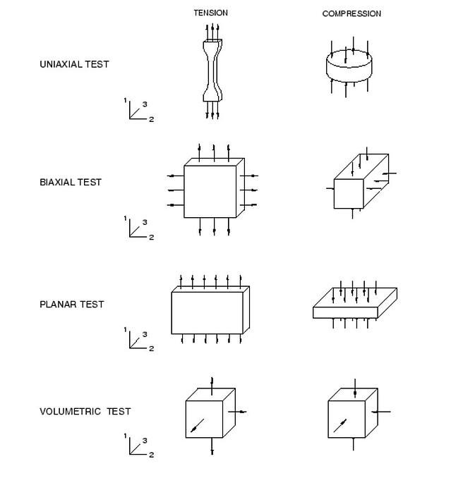
Figure 1: Material testing.

Figure 1 illustrates the deformation modes per test. It is the user’s responsibility to acquire data that are most relevant to the deformation modes that the actual material will endure. This practically means, that if a real-life rubber product is primarily loaded under uniaxial compression,  uniaxial compression test data should be provided in Abaqus for the curve fitting and not uniaxial tension data. Rubberlike materials tend to be softer (less stiff) under tension in comparison with compression.

Also if an actual rubber product is expected to deform up to 600%, it is trivial that relevant testing must be realized up to at least those strain values. This will ensure accurate curve fitting in the region of interest (strain-wise) and consequently realistic results in the finite element model.

Curve Fitting the Test Data

As was mentioned above, when large-strain elasticity is to be modelled,  Abaqus will use the strain energy potential U, in order to relate stresses to strains. Different strain energy potentials are available in Abaqus for hyperelastic materials:

• Polynomial (Moonley, Rivlin, neo-Hookean, Yeoh, reduced polynomial)
• Ogden
• Arruda-Boyce
• Marlow
• Van der Waals

The mathematical form of the strain energy potential U, is given in figure 2.

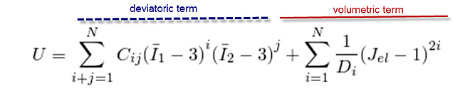
Figure 2: Mathematic form strain potential energy.

This form comprises of two distinct terms, a deviatoric term, modelling the shape change behaviour of the rubberlike material (angular distortion under stress) and a volumetric term (or hydrostatic), modelling the volume change behaviour of the rubberlike material (volume change under stress). This approach is common in continuum mechanics when the stress tensors are considered . This is why those two distinct terms are incorporated in the strain energy potential.  

Then based on the chosen model (e.g. Polynomial, Marlow, Ogden etc.) the above strain energy potential will incorporate different constants (Cij, Di, N) and therefore take a different final form. Based on the different final forms of the strain energy potential, different curve fits will be produced in Abaqus, others fitting effectively to the test data and others less effectively (low correlation). It is the user’s responsibility to choose the most appropriate strain energy potential model based on his/her engineering judgement (e.g. if the actual product is expected to deform between 100 -150 %, the model best fitting the test data for those strain levels should be chosen for the analysis).

This procedure in Abaqus will be depicted and explained next.

Hyperelastic Behavior Modelling in Abaqus

The user must  create a new material and assign hyperelastic properties. The respectful menu is shown in figure 3.

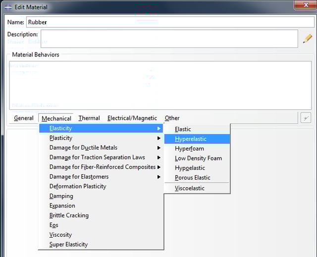
Figure 3: Hyperelastic material property.

Next we can provide available experimental test data, based on the experimental tests performed. This is shown in figure 4. It is noted that for rubber the nominal stress, nominal strain test data should be provided as input. Volumetric Test data are only relevant if compressibility is to be incorporated in the analysis. Alternatively Poisson’s ratio can be input directly . The supported tests are given in figure 1.

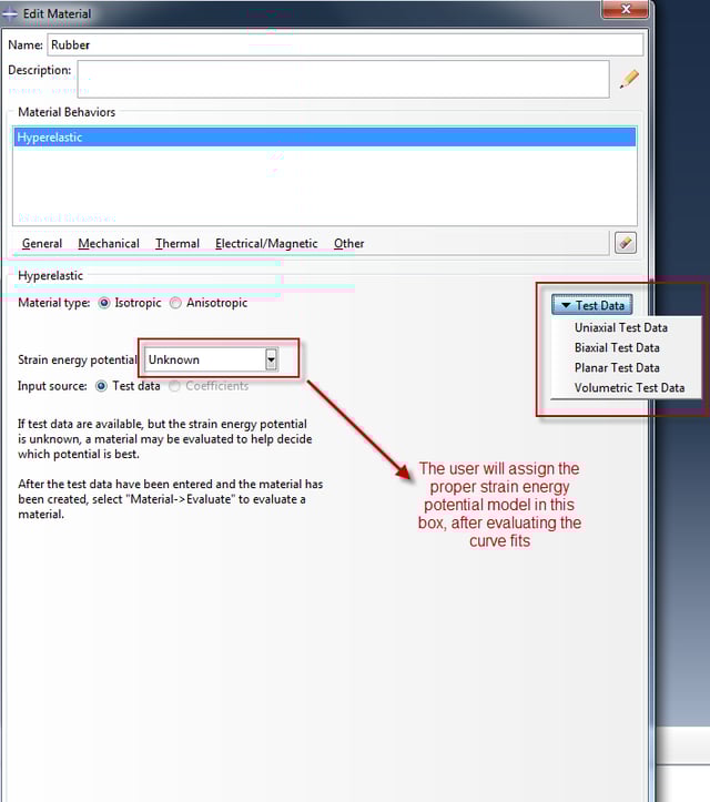
Figure 4: Test data input.

As soon as the test data input is complete, next we need to perform a material evaluation. This is practically the process of curve fitting the test data based on the available strain energy potential models. This is shown in figure 5.

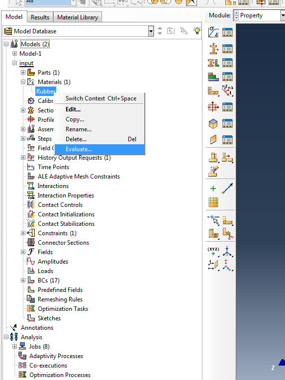
Figure 5: Material evaluation.

On the “evaluate material” menu, we find two tabs. The first tabs allows us to control the test data that will be used for the material evaluation as well as the strain limits for the material evaluation (in case we have test data available for a broad strain range but we are only interested in evaluating our material for a small range). The second tab allows us to choose the strain energy potential model that will be fitted to our test data.  This information is shown in figure 6.

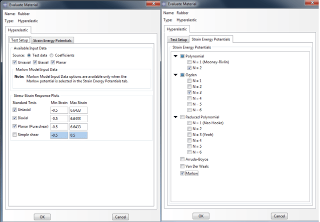
Figure 6: Material evaluation settings.

After the input shown in figure 6 is finalized, Abaqus will perform the material evaluation. Relevant curves will be generated per test type (in the test setup tab-picture 6). The produced curves based on exemplary data are shown in figures 7,8 and 9 for uniaxial, biaxial and planar test data respectfully.

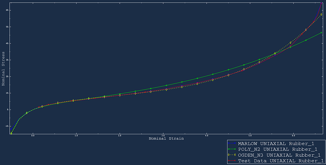
Figure 7: Uniaxial fit.

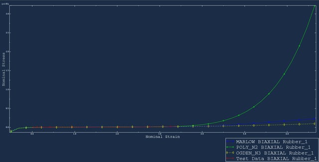
Figure 8: Biaxial fit.

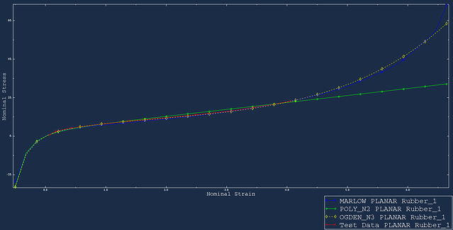
Figure 9: Planar fit.

Relevant function constants of the strain energy potential U can be calculated within Abaqus based only on the provided test data. This is depicted in figures 10, 11, 12 for the polynomial energy function with N=2, the Ogden energy function with N=3 and the Marlow energy function respectfully.

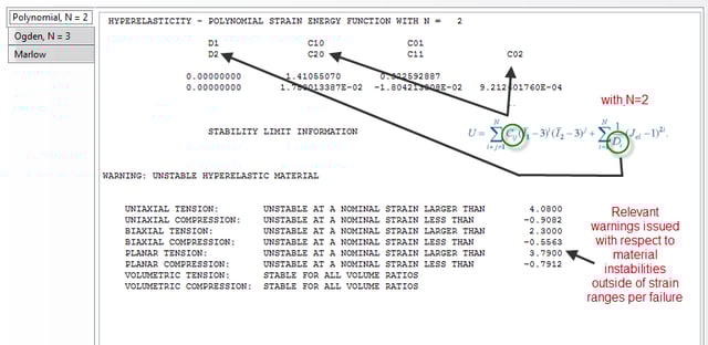
Figure 10: Polynomial fit information.

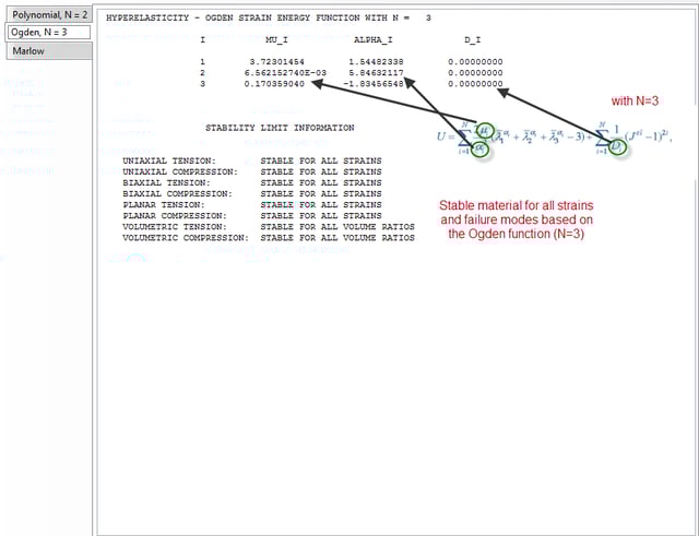
Figure 11:Ogden fit information

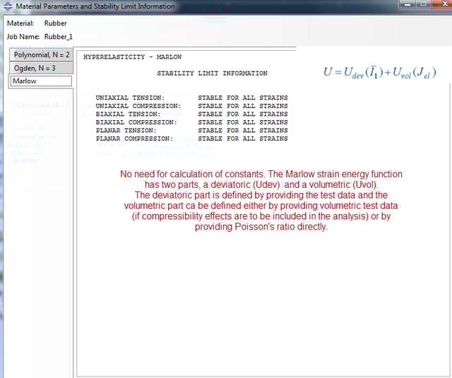
Figure 12: Marlow fit information.

Next step is to choose the strain energy model that best fits our experimental data. As was mentioned above, this is the user’s responsibility.  A good practice for material evaluation overall would be to:

• Check what mode of failure the real-life product is expected to have. Order testing of specimen corresponding to that failure mode.
• Assess the expected strain levels up to which the product is expected to deform. Order testing of specimen at least up to that strain level so that more relevant experimental data are available for input in Abaqus.
• Evaluate the effectiveness of data fitting of different strain energy models, for the failure mode and in the strain range of interest. For example a strain energy model might fit test data more accurately than another but at a different strain range than the one expected for the real product.
• Inspect warnings produced by Abaqus regarding material instabilities outside certain strain ranges. If there is interest for those particular ranges where a material instability is occurring, request more material testing on those ranges so that experimental data become available for a more effective curve fitting. If a material deforms up to strain ranges where it is characterized as unstable, the analysis will not run to completion with no apparent reason (contact will be well imposed, no excessive forces etc.)

When the best strain energy model has been defined by the user’s judgement and analysis needs, this can be selected in the material property tab as shown in figure 13. This will then be material’s stress-strain relationship that will be used for the finite element analysis.

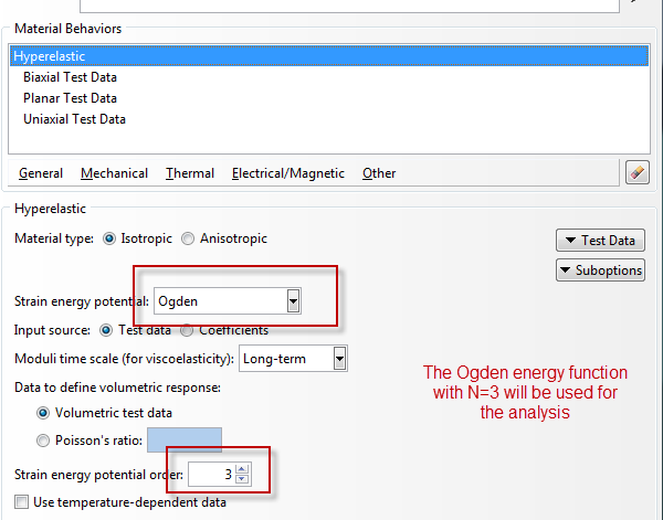
Figure 13: Designated hyperelastic material behaviour.

Finite Element Model

A good practice  when modelling hyperelastic materials is to validate them with use of simplified models. This is of paramount importance also for finite element analysis in general. If your finite element models  are complex in terms of behaviors and non-linearities  and need to incorporate exotic material models, the validity of such parameters can be easily checked  by creating single element models.

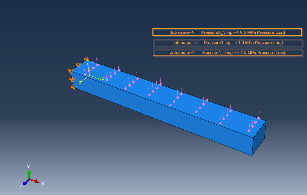
The material behavior that was captured and modelled above, via specific testing on rubber specimens and consequently data fitting, will be reproduced in a single finite element model, a cube of unit dimensions. The finite element  is a linear hexaedron of the hybrid type. As good practice, you should use hybrid elements as often as possible when modelling incompressible or nearly incompressible materials, especially when the material is confined. A video capture of the single element simulation is given below. The type of test can be seen in the legend.