What do you do when you want to find a good design?

Have a brain storm session, come up with different designs, try each one out and choose the best one?

Or let the computer help you, by changing parameters such as dimensions and finding the design that matches the requirements best, possibly using Isight?

While such a parametric optimization is powerful in finding the best variation around a theme, non-parametric optimization can come up with a completely new theme: a new design concept. In this blog, we’ll take a look at non-parametric topology optimization using Tosca and Abaqus.

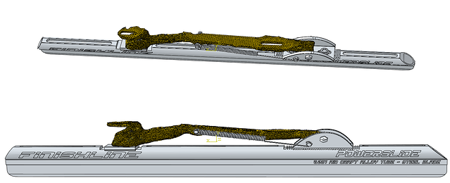
With the Winter Olympics coming up, being Dutch and in need of an applicable topic, we’ll use a Dutch invention; the clap skate (see Wikipedia) as example, and focus on the yellow part in the figure below.

First a regular Abaqus analysis is set up, and then Tosca is used to optimize the topology in this analysis.

Geometry and Mesh

Within Tosca Topology the design variable – what is modified to obtain an optimized solution - is the relative density of the elements in the design domain. Initially all elements have a maximum density. Thus, Tosca Topology looks for an optimal topology by removing material. The starting geometry should therefore correspond to the entire region in which material is allowed. Starting with the current design is not preferred because it steers the result towards the current design concept, while a completely different design may be better. Also, if the design is completely finished it includes many details that are not necessary and require smaller elements during meshing. A coarse shape is therefore preferred.

In order to use the new design in the place of the old one, all connections with other parts should remain intact.

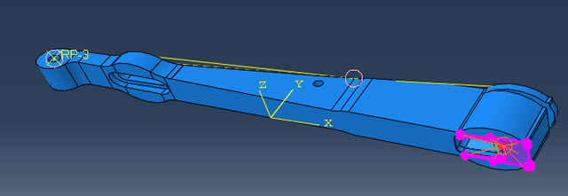
Keeping this in mind, the geometry shown below is used. This is meshed with tetrahedral elements.

Model Set-up

Material properties are defined and assigned. A static, general step is created. Loads and boundary conditions to simulate a person standing on the skate are prescribed: no displacement is allowed at the hinge, though rotation is possible. The region resting on the connection to the blade in the original model is constrained as well:

A force of 800 N (~80 kg) is applied to the top surface using a continuum distributing coupling.

Test Run

With this model, a test run is performed to see whether everything works appropriately and to have an idea of the simulation time. This is not strictly necessary, but because the analysis will be run several times for the optimization, it is a good idea to know it makes sense.

Tosca optimization: Optimization Task

The Tosca optimization can be defined from Abaqus/CAE, using the optimization module. 

First the Optimization Task is defined. In the definition, the type of optimization must be selected (in this case Topology) as well as the region to be optimized (in this case the entire model).

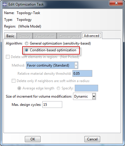
Tosca allows two different optimization algorithms: condition-based optimization and general optimization. General optimization allows many different objectives and constraints (more on what those are later) while condition-based optimization is specifically meant to find the stiffest structure with a certain amount of material. Condition-based optimization will be used here, it is selected in the Edit Optimization Task dialog:

These properties are defined directly in the Optimization Task. Besides this, the Optimization Task also contains Design Responses, Objective Functions, Constraints, Geometric Restrictions and Stop Conditions, similar to the way the model contains Parts, Materials, etc.

Design Response

A design response is a quantity that is measured in the model. It can be used to define an objective function or a constraint. For condition-based optimization the only design responses allowed are strain energy and volume. In this example, a design response is defined for both strain energy and volume. In each case, the sum of values throughout the model in the last step of the current model is used.

Objective Function

The objective function defines what is to be maximized or minimized. In this example, the design response corresponding to Strain energy is minimized, the only allowed option for condition-based optimization. This is equivalent to minimizing compliance, or maximizing stiffness. Therefore, this objective function ensures optimization towards the stiffest structure.

Constraint

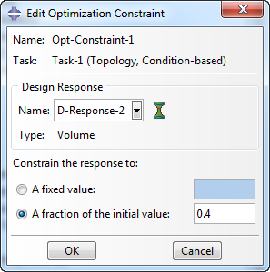
Constraints put bounds on the solution space. If only an objective function requiring a stiff structure would be present, then having maximal density throughout the model would be the optimal solution, as the total stiffness of the structure is highest then. This is not intended: we are looking for the stiffest structure using a certain amount of material. This is where the constraint comes in. For condition-based optimization the only allowable constraint is a prescribed volume. In this case, the volume is constrained to be 40% of the initial volume.

Geometric Restrictions

Though not required for running the optimization, defining geometric restrictions is often useful. They can be used to filter out topologies that are unwanted or unmanufacturable. In this case, two types of geometric restrictions are defined: frozen areas and demold control. In the frozen areas, material can’t be removed. Regions that are to be connected to other parts are frozen (see image below), so the connection will still be possible after optimization.

Different demold options are possible. In this case ‘demolding at the region surface’ is selected. With this option, material is only removed from the outsides, so holes will not develop internally.

Optimization Process

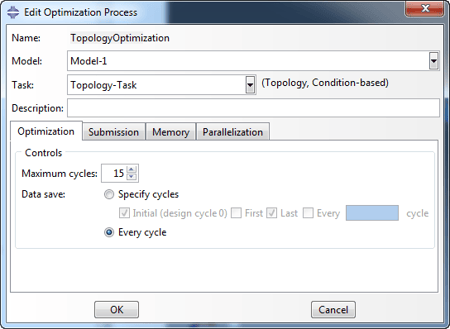
Now that the optimization task defined, the next step is to define an Optimization process. This is similar to creating a job, once the model is defined. In the model tree, Optimization Processes are located under ‘Analysis’, as Jobs are. The Optimization Process is set to refer to the previously created model and task. The maximum amount of cycles is also specified. By default this is 15, so (at most) 15 analysis jobs will be run on the model.  

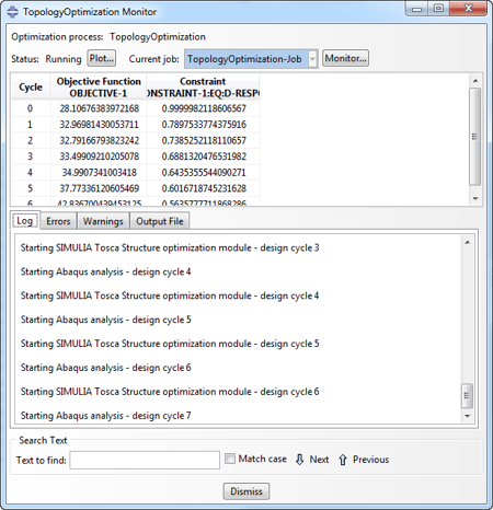
The Optimization Process is then submitted and monitored as a regular Abaqus job. In the monitor window the values of the objective function and the constraint are shown per design cycle:

Of course it takes time to run 15 analyses.

Results

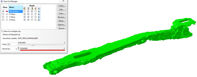
The outcome of the optimization can be viewed in Abaqus/CAE, after the results of the different analyses are combined. The resulting geometry can be visualised by making a view cut, at an isosurface of the MAT_PROP_NORMALIZED variable, by selecting Opt_Surface. The MAT_PROP_NORMALIZED variable gives the calculated relative densities.

The evolution towards the final design is shown in the movie.

The optimized topology can be extracted for further analysis, either as Abaqus input file, or as STL. In this case, an .inp is written. The part is imported and placed in the assembly, instead of the original part (Figure 11). It nicely connects to the existing parts, because the relevant holes were made in the original part and these regions were kept frozen.

Conclusion

In conclusion, Tosca’s condition-based topology optimization can be used to find the location of a specified volume of material that optimizes stiffness under a specified loading. Though the terminology can be confusing at first, setting up an optimization is actually quite straight-forward using Abaqus/CAE.