

Posted by Christine Obbink-Huizer
Table of contents
In this blog, we’ll take a look at an air spring (Figure 1). This device is used for vibration isolation as well as suspension, for example in heavy weight vehicle applications.
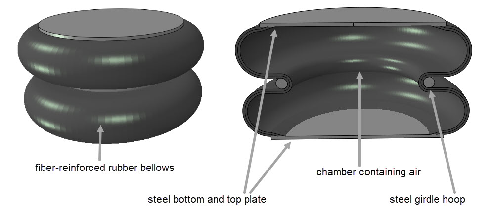
Figure 1: Example of an air spring.
The example shown here consists of a convoluted bellows (two convolutions), with steel plates on each end. In practice, one to three convolutions are used. The bellows is made of rubber that is reinforced with fibres. A steel girdle hoop helps to keep it in shape when it is filled with compressed air.
Compared to a mechanical leaf- or coil-spring an air spring has the advantage of being adjustable: by changing the pressure inside the air spring, the spring characteristics change. This offers additional comfort to the user. Furthermore, the length of the air spring can be adjusted by adding or removing air. Because of this, air springs can be used for levelling and to adjust height.
As explained above, the behaviour of such an air spring depends not only on the geometry, material properties and reinforcement choices, but also on the air that is contained within. In this blog we will simulate this air spring, including its air chamber, and look at how the force-displacement behaviour is influenced by changing the internal pressure.
Geometry
The geometry is shown in Figure 1. For simplicity, an axisymmetric approach is used. We will only look at the axial force-displacement behaviour here, so this is sufficient. It is possible to extend this to no-axisymmetric cases later on, for example to see how the air spring responds to non-axial loading.
To model reinforcements, a layer of reinforcements is included in the middle of the thickness of the bellows (Figure 2). It includes fibres at an orientation of +/- 15 degrees with respect to the longitudinal direction. These are balanced, to maintain axisymmetry.
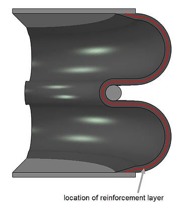
Figure 2: Location of reinforcement layer.
This is done using the rebar option in Abaqus. The axisymmetric face is partitioned, to obtain an edge at the location of the reinforcement layer. A skin is defined at this edge. A surface section including the rebar is assigned to the skin. In the rebar definition, the material of the reinforcements, the area per bar, the spacing of the bars and the orientation angle are defined. In the case of axisymmetric shells, it is not necessary or even possible to define a coordinate system for the rebar angle. Angles are defined with respect to the r-z plane. With an angle of 0 degrees, the fibres lie in the r-z plane (the plane that is explicitly modelled). With an angle of 90 degrees, the fibres are perpendicular to this, so in the circumferential direction.
Material
The top and bottom plate are considered rigid. Rubber material properties (hyperelastic Mooney-Rivlin) are used for the bellows. Steel properties are used for the girdle hoop and fibre reinforcements. The air inside the air spring is considered to be an ideal gas, with the molecular weight of air (0.0289).
Fluid Cavity
The air is included in the analysis using a fluid cavity. This allows a pressure-volume relationship (in this case that of an ideal gas) to be applied to a surface. The surface used is the internal surface of the bellows and top and bottom plates, as shown in Figure 3.
Figure 3: The surface used to define the fluid cavity.
Within a fluid cavity, the pressure is assumed to be constant. A pressure can be prescribed as a boundary condition to the fluid cavity. In this case, air can flow in or out of the cavity, to obtain this pressure. When no pressure boundary condition is active, then the cavity is closed; no air can flow into it, or out of it. More complex inflation options are available as well, for example to model airbags.
Within Abaqus, fluid cavities are a type of interaction. A surface and a reference point must be defined. For (axi)symmetric cases, the reference point must lie on the axis of symmetry (even if this is outside the fluid cavity itself for axisymmetric problems). The fluid cavity definition refers to an interaction property that defines the fluid cavity properties. Within it, you can choose whether the fluid cavity is hydraulic or pneumatic. For pneumatic fluid cavities, such as the one used here, the ideal gas molecular weight must be specified.
To use this option, the absolute zero temperature and universal gas constant should be defined as model attributes.
Loads and Boundary Conditions
For each analysis, three steps are simulated. During the first step, the air spring is pressurized. Both end plates (top and bottom) are fixed during this step. During the second step, the top plate is moved to reach an axial compression of 25%. During the last step, the top plate is moved to reach an axial extension of 40%. This allows us to draw a force-displacement graph.
These steps are performed for three pressure levels: 1, 2, 3, 4 and 5 bar so that the effect of pressurization can be shown.
Additionally, the pressure is increased while allowing the air spring to expand. This shows how pressurizing the air spring can be used for levelling.
The analyses are performed using Abaqus/Standard.
Results
As expected, the length of the air spring increases, as the pressure is increased:
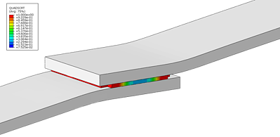
The deformation during the compression-extension test is shown below:
When plotting force vs displacement for all pressure levels, then we observe a larger force, as well as a higher spring stiffness force as the pressure level increases (Figure 4).
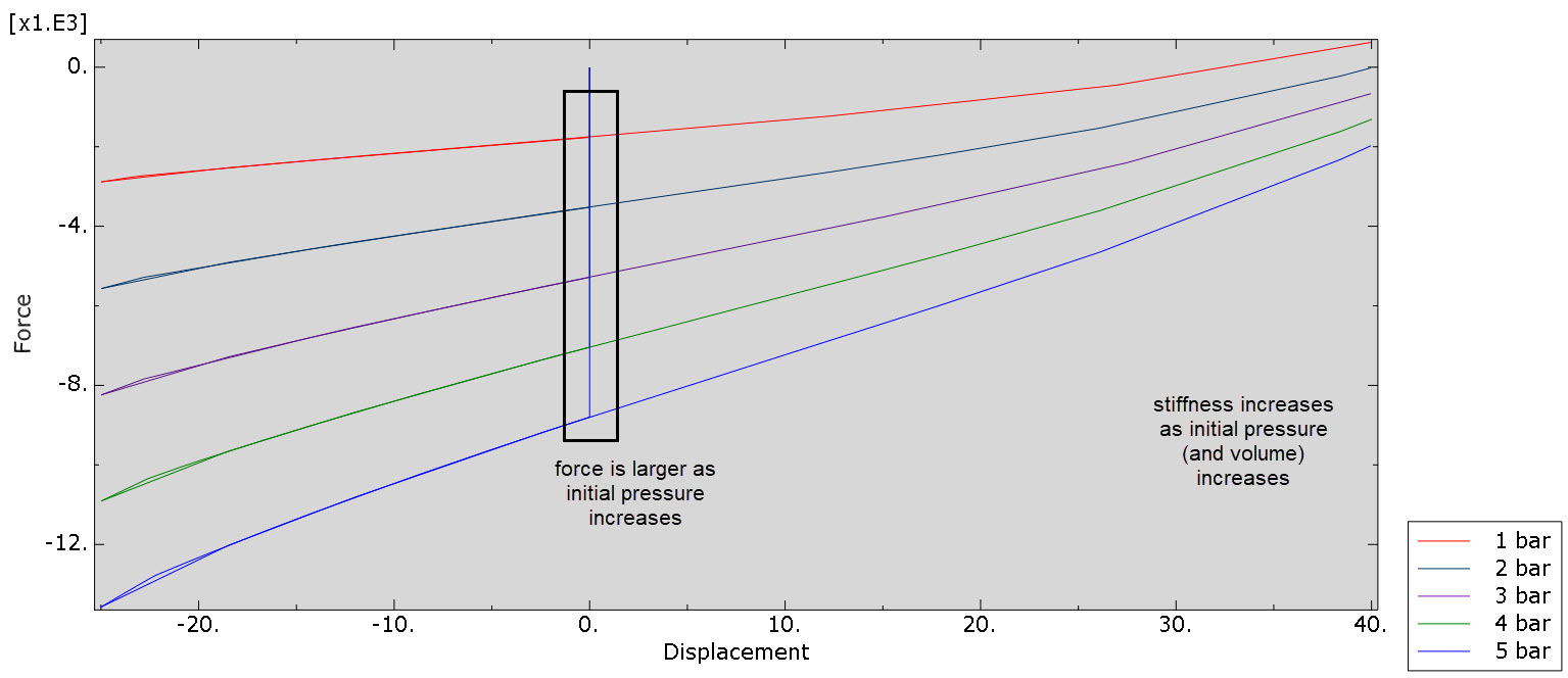
Figure 4: Force-displacement relationship for different initial pressure levels.
Conclusion
I have shown a way to model an air spring, using the fluid cavity option in Abaqus. This is a straight-forward way to include rather complex behaviour. We have currently looked at the axial force-displacement relationship for different initial pressures. Many other things can be investigated as well, such as the influence of the orientation of the fibres, or more complex loading conditions.


TECHNIA Simulation provides top tier FEA, Non-linear, and Advanced Simulation Software, Training, and Consultancy. Our dedicated team of more than 65 Simulation experts across 16 countries advise and support your innovation with a wealth of specialist knowledge and experience.
About TECHNIA- Related news and articles straight to your inbox
- Hints, tips & how-tos
- Thought leadership articles

Helping you find the information you’re looking for. Discover webinars, events, FAQ's, case studies and tutorials.
VIEW HUB