
Posted by Paul Bolcos
Table of contents
In this blog post I thought we would take a small dip into modeling fracture and failure with Abaqus. In conventional FEM methods for crack propagation, the initial crack location needs to be predefined. This is not necessary when using extended Finite Element Method (XFEM). XFEM uses enrichment terms to the normal displacement interpolation to describe the crack behavior.
We've previously discussed about modeling cracks using conventional approaches and XFEM. I thought it would be nice to revisit this topic, focusing mainly on XFEM approach on a familiar geometry: the hip implant from the previous geometry and meshing blog.
Introduction
Conventional fracture modeling only permits crack propagation along predefined boundaries. However, if we want to model bulk fracture and allow the crack to be located in the element interior, XFEM comes in handy.
More importantly, there are some advantages when it comes to the crack itself: 1) No need to specify the crack path and initial location; 2) Mesh is generated independent of the crack; 3) No need to partition the geometry at the crack location; though the mesh density should be high enough.
Model Setup
Geometry, Mesh
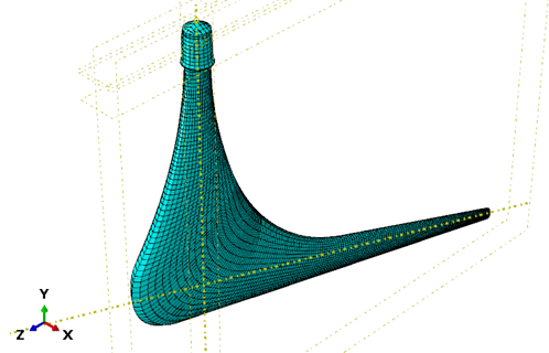
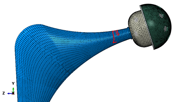
The previous hip replacement geometry was used. This was then partitioned so that we could obtain a hexahedral mesh on the part. To accurately model the crack propagation path, a denser mesh would be needed for this part, but for illustration purposes, it should be enough.
Material Properties, Damage Model
Ideally the implant would be made of a CoCr or Ti6Al4V alloy, but fracture criteria are scarce. To illustrate the principle of XFEM, we used generic steel properties: E=210 GPa, ν=0.3, ρ=7850 kg/m3.
To model crack propagation in Abaqus, we need to describe the damage initiation and evolution behaviors. For damage initiation, several criteria are available: maximum nominal stress/strain, quadratic nominal stress or maximum principal stress/strain. In each case, damage is assumed to initiate when the stress/strain satisfy the input damage criteria. In this case maximum principal stress (MAXPS damage) was used. This has the advantage that the crack plane can be perpendicular to the direction of maximum principal stress making it solution dependent. For this case, once the maximum principal stress exceed a value of 400 MPa. 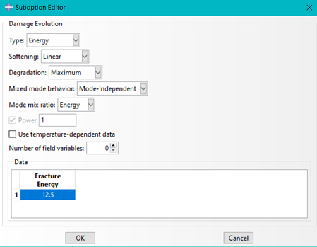
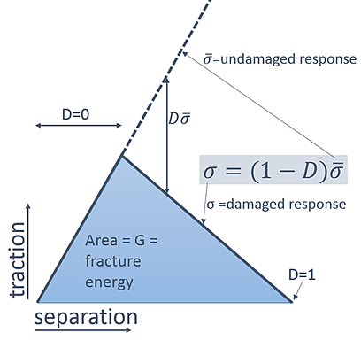
To model how the material changes due to damage, we need to define damage evolution. This is modelled with a scalar damage parameter (D). The range is between 0 (no damage) and 1 (complete failure). The stress calculated if there is no damage (![]() ) is then multiplied by (1-D) to calculate stresses including damage (σ). Without damage, this lead to undamaged response; with complete failure, the stress is 0. In between, there will be a fraction of the stress (Figure).
) is then multiplied by (1-D) to calculate stresses including damage (σ). Without damage, this lead to undamaged response; with complete failure, the stress is 0. In between, there will be a fraction of the stress (Figure).
![]()
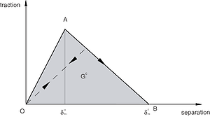
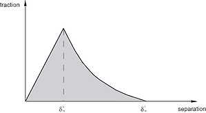
We can define the evolution in terms of maximal displacement (δm-δn below) or fracture energy (G). Then we can specify the "softening" behaviour: i.e. how the traction-separation graph evolves from damage onset (A) to complete failure (B) and it can be linear or exponential. It is also possible to take into account mode-mixing with BK law, power lab or tabular data. In this example, I used the linear and exponential softening.
To make calculations easier, there is also a damage stabilization term. It uses viscosity coefficients to improve the convergence as the material fails. This coefficient should be small so that it doesn't influence the final result.
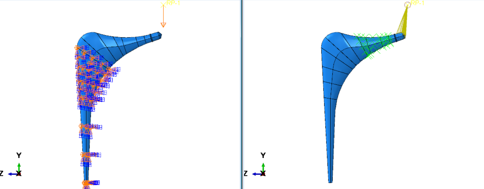
Boundary Conditions, Loads, Interactions
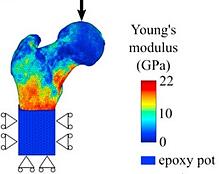
In lab mechanical tests, the femur main body is kept fixed, while a top load (force) is applied. An example of this, plus an XFEM based method to predict crack initiation in patients hip using Abaqus can be found here. In this case, we used a similar setup.

This is also where we define the XFEM Crack. In the Interaction Module under Special → Crack we can define an enriched region. In this region the crack will initiate and propagate. The XFEM-based cohesive segments method can simulate crack initiation and propagation along an arbitrary, solution-dependent path in the bulk materials. To represent the discontinuity of the cracked elements, phantom nodes are introduced. Without going into too many details, essentially we can have a crack propagating in between an element, effectively splitting it into two parts. A complete description of how the enrichment function works, how the phantom nodes work can be found in the manual under Abaqus → Analysis → Analysis Techniques → Modeling Abstractions → Modeling discontinuities as an enriched feature using the extended finite element method → References (online link for Abaqus 2021).
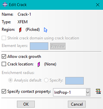
This enrichment zone can be either an entire part or just a specific subset.
Solution Controls, Output Requests
As this is a very discontinuous and difficult problem to obtain a converged solution, we need to modify the solution controls. In the step module, select Other → General Solution Controls → Edit → Step (in which the solution control will be edited). Press continue when the warning message is displayed. In the time incrementation tab, check/enable the discontinuous analysis option (allows Abaqus to do more iterations before checking if the solution is going anywhere); In the first More Tab, increase the parameter IA from the default 5 to ex. 20 (allows Abaqus more attempts before aborting, especially with large cut-backs)
Results
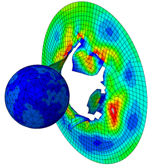
The animation below shows the crack initiation and propagation for the femoral stem.
If we superimpose the crack location and propagation path on the full THR implant we get the image below.
Discussion
Even though we are using steel instead of CoCr, the crack location is not to dissimilar to the the experimental crack investigation by Ryniewicz et al., where a real femoral stem. In their specimen, there is also an additional smaller fracture near the failed region. 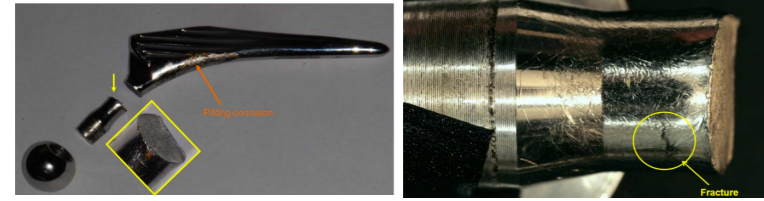
XFEM is a nice tool, but generally we're more interested if there will be a crack forming in a specific region and perhaps more important IF the crack will propagate. For that purpose the more traditional approach of modeling cracks using J- integrals or stress intensity factors (K) may be sufficient (A brief overview by Christine shown here).
So when would XFEM be more important? First, when we have no idea where the crack tip will be located. A second would be to match FE model predictions to real physical specimens. If the fracture behavior is accurate, this could replace physical testing. You could cycle through several designs and optimize the final product.
Discover More
Paul recently presented 'Subject-specific Finite Element Models to Identify Patients at Risk of Osteoarthritis' at SIMULIA RUM 2021, view the session on demand via the link below.

TECHNIA Simulation provides top tier FEA, Non-linear, and Advanced Simulation Software, Training, and Consultancy. Our dedicated team of more than 65 Simulation experts across 16 countries advise and support your innovation with a wealth of specialist knowledge and experience.
About TECHNIA- Related news and articles straight to your inbox
- Hints, tips & how-tos
- Thought leadership articles

Helping you find the information you’re looking for. Discover webinars, events, FAQ's, case studies and tutorials.
VIEW HUB