Use Abaqus to Simulate Additive Manufacturing – Printing a Hip Implant

In finite element analysis, traditionally we define the geometry at the start of the analysis and assume that while it may deform, the amount of material stays the same. For additive manufacturing, this is clearly not the case: material is continuously added. If we look at the thermal aspects of things, we also see a constantly changing problem: over time heat is added at different points in space; and the outer surface, where heat loss occurs, changes over time. Specific capabilities are therefore needed to efficiently set-up the simulation of problems that continuously change, such as the additive manufacturing process.

Already for some time Simulia is working on user subroutines, keywords, data structures, and a plug-in that make the simulation of additive manufacturing more straight-forward. From Abaqus 2019 FD01 onwards, additive manufacturing process simulation is included in the manual (link requires dsxclient customer login details) (Figure 1), indicating that this is becoming more mainstream. It therefore seems to be a good time to take a closer look at the capabilities.

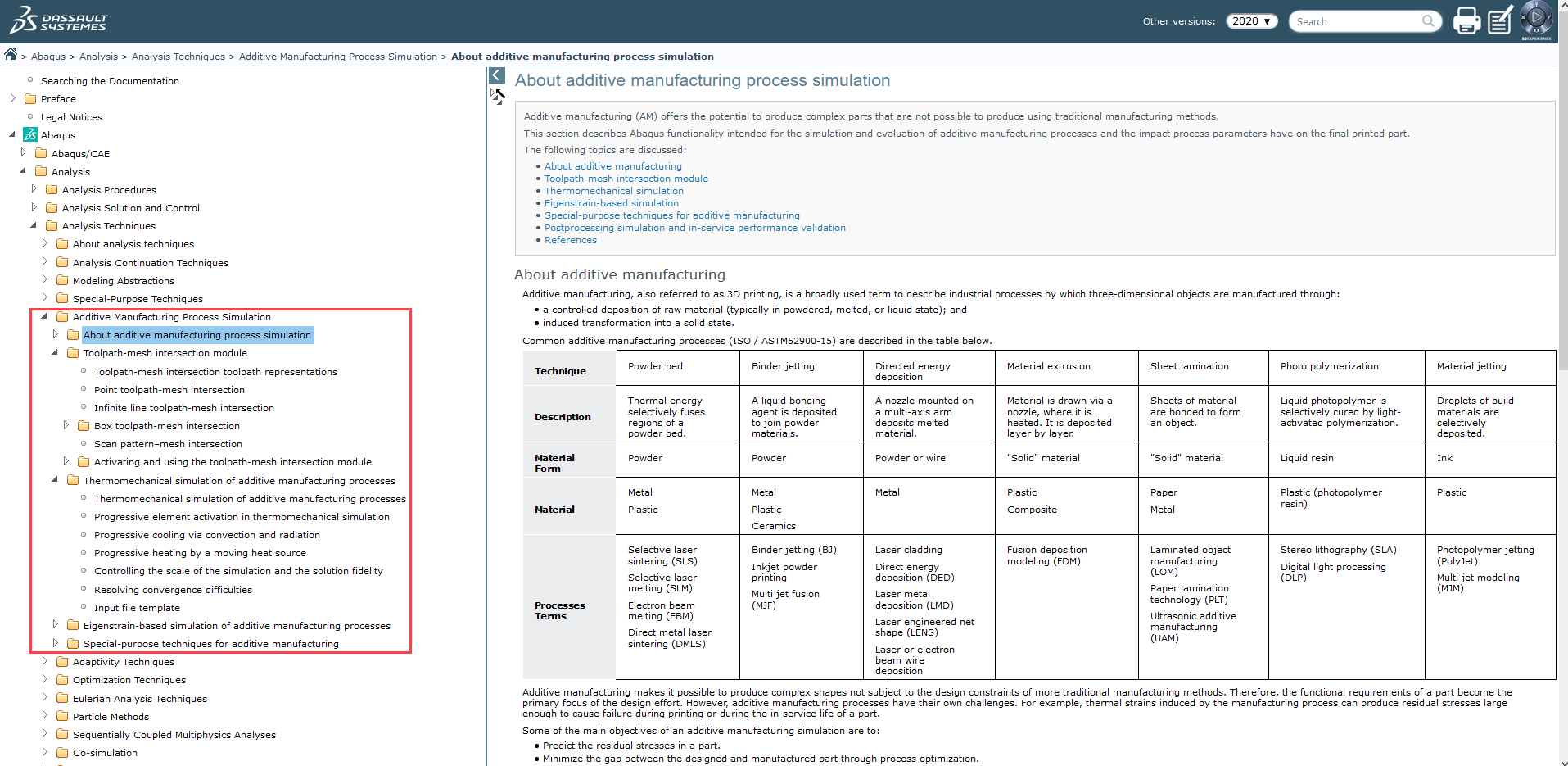
Figure 1: The manual now includes an extensive section on additive manufacturing.

At the core of the additive manufacturing simulation capabilities is the toolpath – mesh intersection module. This is used to determine which elements have intersected with a path that is defined in time and space, for example the path of a tool. Without this, it is only possible to add elements at the start of a step, and the elements that are to be included need to be defined explicitly. The toolpath – mesh intersection module allows for a much looser coupling between the toolpath and the rest of the model. This makes the model set-up simpler and less time-consuming; you don’t need to define as much steps, surfaces, boundary conditions, etc.

Example: Hip Implant With LDED

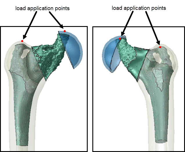
As an example, I will use the optimized hip implant design (Figure 2) that was the output of a previous blog  .

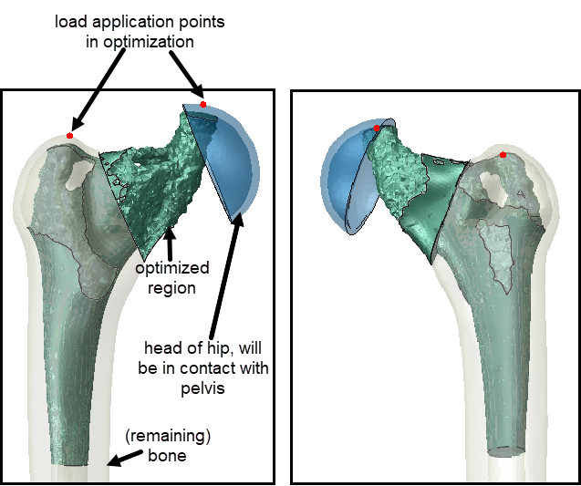
Figure 2: The optimized hip implant design, as described in the previous blog. The additive manufacturing of only the green part will be simulated.

I will use this geometry as an example for additive manufacturing using Laser Direct Energy Deposition (LDED). Here, a part is built up by depositing melted material on the workpiece, layer by layer (Figure 3). Both the material addition and the energy input are taken into account.

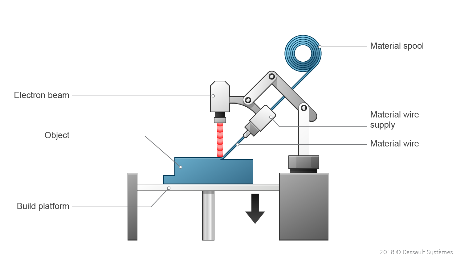
Figure 3: The additive manufacturing process that is used as example here (LDED). Taken from https://make.3dexperience.3ds.com/processes/directed-energy-deposition.

It is also possible to use the additive manufacturing capabilities for other techniques than LDED: the additive manufacturing capabilities are set up in a general sense. Many things are possible, but some require you to write your own user subroutines. The example we have chosen here uses built-in options, so we can show the concepts without making things more complex than necessary.

Preliminaries

Two models are defined in Abaqus/CAE: a thermal and a structural model. These include the geometry, mesh, material properties, boundary conditions and predefined fields to define the initial temperature and apply the temperature output from the thermal model to the structural model. The additive manufacturing process is not yet defined. The rest of the blog focuses specifically on this.

AM Modeler

The additive manufacturing capabilities allow for material addition and sequential thermal mechanical analysis. Since the problem changes in time and is temperature dependent, a lot of data is needed, that will be used by user subroutines. Various data structures have been developed so that the data can be sent to the user subroutines in a rather easy manner. This is based on keywords in the input file. A plug-in is available to guide the definition of the keywords from the CAE. Here, I want to explain the different data structures in a general sense, as well as provide a specific example in which things are defined using the plug-in. More information on the plug-in and how to obtain it can be found in QA000000575 in the knowledgebase, (link requires dsxclient customer login details).

Once the plug-in is installed, the AM modeler can be made visible by selecting Plug-ins --> AM Modeler (Show/Hide). This will give an extra tab, along with the Model and Results tabs. Right-clicking AM-Model allows you to create an AM Model. One of the options that can be selected is the ‘Abaqus builtins’ process type (Figure 4). If this is selected, then the predefined types will be available, otherwise you need to define the types yourself. We will use predefined types here.

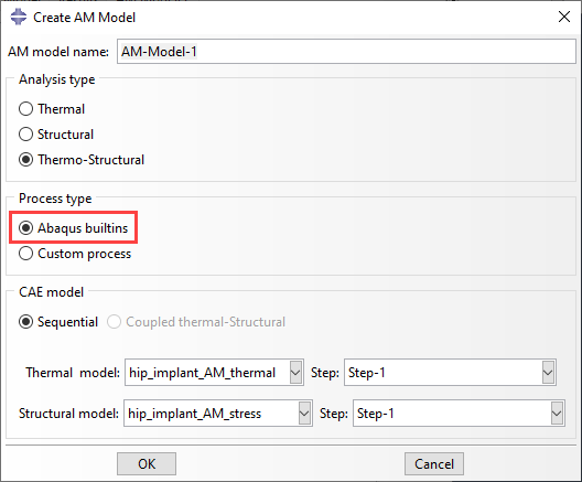
Figure 4: Creating an AM Model. By selecting ‘Abaqus builtins’ as indicated here, the predefined types will be available.

An AM model is visible in the AM modeler tab (Figure 5). It has different sections: Data Setup, Model Setup and Simulation Setup, of which the Data Setup is most extensive. Types for different data structures are mentioned, including the Parameter table, the Property table and the Event Series. We will take a closer look at these data structures.

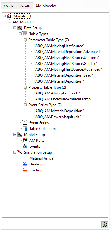
Figure 5: The AM modeler tab. Predefined types are shown here.

Event Series

To define data in a time and space dependent manner, the event series is developed. This is basically a combination of an amplitude curve and a path. The main structure is

time_1, x_1, y_1, z_1, field_value1_1[, …]

time_2, x_2, y_2, z_2, field_value1_2[, …]

The amount of field values that is to be provided, depends on the type of event series: within the event series type definition, the amount of field variables is defined.

Event series types can be defined by the user, but there are also predefined options. The type will then start with "ABQ_AM". In our example of LDED event series are used to define the material deposition path and the laser path. One event series is used for the material path and another for the laser path. Predefined types are used. Each event series has one field value. For the material path this is 1 or 0 and represents material being deposited (1) or not (0). For the laser path, this represents the power of the laser. For two subsequent rows, the field value of the first row is held constant until the point on the second row is reached. An example of defining a material deposition Event Series from the AM modeler is given in Figure 6.

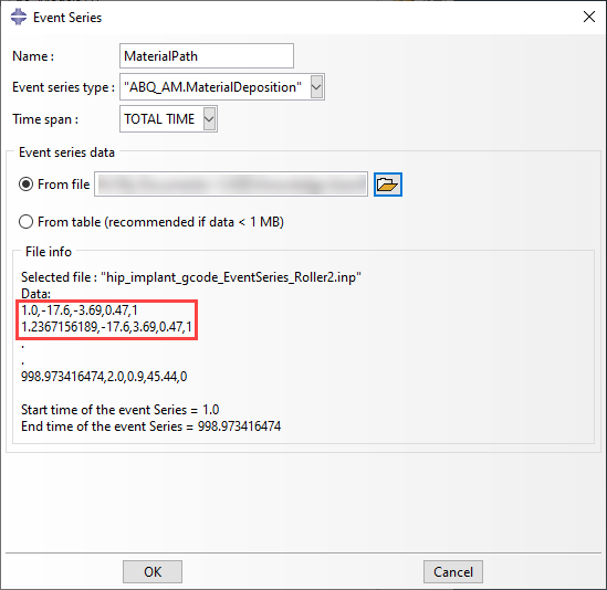
Figure 6: Event Series definition, in this case via a separate input file. Part of the actual data is shown in the red block.

To obtain the event series data for this example, I used the approach suggested in the attachments of QA000000575 in the knowledge base: I have generated gcode using replicatorG and converted this to event series using the supplied script called generateEventSeries.py.

Parameter Table

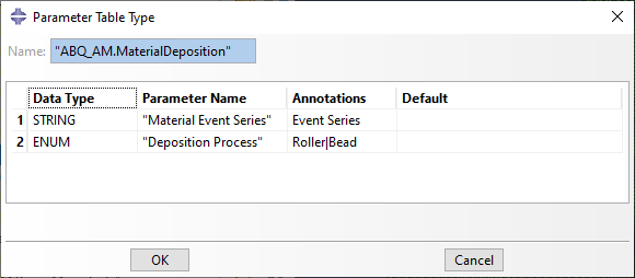
A Parameter Table is used to group process specific parameters that do not depend on time, space or material state. The amount and type of parameters that are included in the parameter table, is determined by the Parameter Table Type. For some common additive manufacturing processes, the required Parameter Table Types are predefined. An event series can be a parameter in a parameter table. In our LDED example, we will use several predefined parameter table types, such as “ABQ_AM.MaterialDeposition” (Figure 7).

Figure 7: An example of the definition of a Parameter Table Type. For all parameters included (2 in this case), the data type, parameter name, annotations and a default value can be specified.

In the AM modeler, you typically do not need to define a Parameter Table separately but do this as part of a Table Collection. More on Table Collections later.

Property Table

Property Tables are used to define dependent parameters. The parameters can depend on temperature, field and state dependent variables. Parameters such as material properties and a film coefficient can be defined this way. An example of a Property Table Type is "ABQ_AM.AbsorptionCoeff", the definition in the AM Modeler can be seen in Figure 8. This is an example of a predefined Property Table Type.

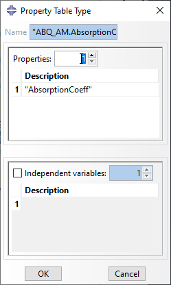
Figure 8: The definition of the “ABQ_AM.AbsorptionCoeff” Property Table Type in the AM Modeler.

Similar to Parameter Tables, you typically do not need to define a Property Table separately, but do this as part of a Table Collection.

Table Collection

Table Collections are containers that encapsulate Parameter Tables and/or Property Tables. This way, they can be grouped together for reference in user subroutines. For our LDED example, we will use two Table Collections. One will describe the material deposition, the other the heat input. In the AM Modeler, we can create Parameter Tables and Property Tables according to the previously defined Types (in this case the predefined ones). An example of defining a Parameter Table of type “ABQ_AM.MaterialDeposition” is given in Figure 9. Multiple boxes can be ticked, to define different types of Property Tables and Parameter Tables in a Table Collection.

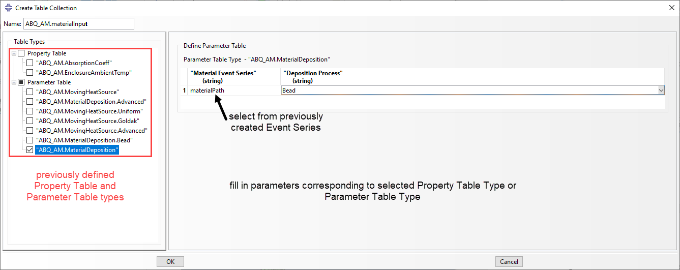
Figure 9: Defining the material input Table Collection. Here, the Parameter Table of type “ABQ_AM.MaterialDeposition” is filled in.

Model Setup

Obtaining the data and defining it, is typically most work. Once this is done, we can select the parts to be included in the AM analysis via Model Setup --> AM Parts. It is also possible to visualize the Event Series. You can then see the path that is used in the analysis on the geometry (see Figure 10 for an example).

Figure 10: The ‘View Events’ option in the AM Modeler, showing the material path between t=20 and t=30 seconds.

Simulation Setup

Finally, the Table Collection used to define the material arrival and the Table Collection used to define the Heating are specified. It is also possible to specify cooling via convection and/or radiation. This will automatically be applied to the current outer surfaces then.

Summary of AM Modeler Interface

We have now gone through the entire AM Modeler interface. A visual summary is given in Figure 11.

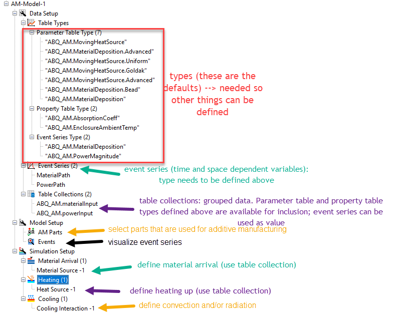
Figure 11: The AM Modeler interface, indicating what is defined where.

Running the Analyses

The AM modeler will ensure the keywords that are relevant to additive manufacturing are included in the input files when the jobs are run. The thermal job is run first, followed by the stress job.

Results

A movie of the results is shown below:

We see material being added during the analysis, temperature changes due to the heat flux, and stresses developing due to the temperature changes.

Comparison to *model Change Option, As Used in the AWI

The capabilities described here use *ELEMENT PROGRESSIVE ACTIVATION. This activates the toolpath – mesh intersection module. An alternative way to activate elements during an analysis, is to use *MODEL CHANGE. This approach is used in the Abaqus Welding Interface (AWI).  With *MODEL CHANGE all geometry that is to be included at any time in the model is defined from the start, and elements can be activated or deactivated during the analysis (see this blog). It is not possible to change which elements are activated during the step, so gradual activation of different elements typically requires a lot of steps. The outer surface changes when elements are activated, so in thermal analyses regions of heat loss tend to vary. This requires defining a lot of different surfaces, and different interactions to consider the changing surfaces. All in all, we are talking about models with many definitions that are time-consuming to set up. The Abaqus Welding Interface is intended to make this process easier (see this blog for more info).

For additive manufacturing, the amount of material that needs to be added is more extensive than for a typical welding analysis. This makes an analysis based on *MODEL CHANGE even more extensive and this strategy feels more like a workaround than that the software is meant to simulate the process of material addition.

As mentioned before, with the *ELEMENT PROGRESSIVE ACTIVATION approach we can define progressive element activation within a step based on a geometrical path and time instead of having to explicitly define when each (set of) element(s) is activated. The coupling between the toolpath and the rest of the model is therefore much looser. Because of this, refining the mesh or reducing the time increment size has a more gradual effect when using *ELEMENT PROGRESSIVE ACTIVATION compared to *MODEL CHANGE. For example, if the time increment is reduced when using *MODEL CHANGE (AWI), then the same blocks of material will still be added at the same times, because material activation is explicitly defined between steps. If the time increment is reduced when using *ELEMENT PROGRESSIVE ACTIVATION, then the material will be added more gradually; less elements will be activated per increment. An example of this is given in the movie below, where for part of the analysis either a time increment of 1 is used (left) or 0.01 (right). The change in time increment is the only modification made to the model, and the activated elements are nicely interpolated.

Conclusion

• With these additive manufacturing capabilities, it is much simpler to simulate problems where material and heat are added in a time and space dependent manner that with *MODEL CHANGE.
• Because user subroutines are used, a lot of user control is possible.
• The predefined options allow more ease of use for common cases.
• Data structures are defined specifically for this.
• The AM Modeler can help to properly define everything.
• Obtaining and defining the required data can take most effort.
• Though it may take some effort to understand how to use this, I expect it is definitely worth the effort if you want to simulate additive manufacturing or similar processes.