 Advanced Simulation


Abaqus is known for being a general-purpose suite of finite element tools, encompassing both implicit and explicit solvers. This allows almost all classes of structural problem to be tackled within the same environment and toolset, from linear static models all the way up to large crash simulations with every kind of nonlinearity possible throughout the transient solution.
To compliment this, there is a wealth of diagnostic information available at every stage of model build, solution and post-processing for any given simulation. This helps the analyst to confirm both that the model is creating the abstraction of reality that they intended, and that the solver is interpreting that model correctly and creating appropriate, viable and useful results.
Most of the available solver technology can be defined through the Abaqus/CAE interface (‘CAE’ in this case standing for ‘Complete Abaqus Environment’), but the word ‘most’ in this sentence is important, as there is useful functionality in the solvers that can only be accessed outside of the Abaqus/CAE environment.
One such example is the ‘unconnected regions’ job execution option, which can only be accessed if the simulation is executed manually from a command line. If the user executes a simulation from within the ‘Job Manager’ of Abaqus/CAE (as shown in Figure 1), the options are limited to:
- Write the Abaqus input deck, but not launch the solvers.
- Perform a ‘Data Check’ on the model, which submits the input deck to the solver but only up to the point that input syntax is checked and the system matrices are assembled .
- Submit the model for full analysis through Abaqus/CAE.

Figure 1 – Analysis execution options through the ‘Job Manager’ in Abaqus/CAE
However, if only the Abaqus input deck is written from Abaqus/CAE, the user has the ability to execute the job manually through the command window of the PC’s operating system.
If the job is executed at the command line, then additional options for the solve can be defined which are not available through Abaqus/CAE. As mentioned, one of these is the ‘unconnected_regions’ option which must also be used in combination with the ‘datacheck’ option as well.
Why is this useful? Given the capabilities of Abaqus, there are clearly scenarios where we might want to build a model of an assembly of components where we are interested in when and how these components interact with each other. In these cases, there will be regions of the model which are contiguous, but these may be distinct and unconnected from other regions: the facility by which load will be transferred between these regions could then be a contact interaction which will engage at some point in the loading history. As an initial phase of the solution of any analysis, the solver first works through the model to identify how many regions are directly connected together. This could either be through regions of contiguous mesh or other features of the model which force degrees of freedom to be constrained between elements, other than at shared nodes (tie constrains, couplings or connector elements for example).
Having done this check, a simple message summarising the findings is issued towards the top of the .msg file associated with this job, which may look something like that shown in Figure 2.
![]()
Figure 2 – Example message identifying the number of unconnected regions.
For simple models, the number of unconnected regions the analyst is expecting may be obvious and a message such as this matches the expected number and simply confirms the model is correct. But in more complex assemblies the number of unconnected regions in the model could be harder to predict, and the reported total may be a result of a modelling error leading to the solution failing to converge (an unconstrained region of the mesh subjected to a gravity loading, for example).
Therefore, it is often very useful to be able to visualise the unconnected regions of mesh that the solver has identified, either to simply confirm that the model is assembled correctly or to track down convergence issues if the solution is not behaving as intended.
To access this capability, simply create the Abaqus input deck for the model you want to check and execute at the command line using the options shown in Figure 3. This activates the ‘unconnected_regions’ option during initial model processing by the solver and creates internal element sets of each contiguous section of the mesh.
Note again that this must be used in conjunction with the ‘datacheck’ option, and therefore the solution will intentionally terminate at the point the model checks are done and will not proceed to actually solving the analysis. It is also worth saying that the ‘datacheck’ phase of the solution is non-parallelisable, so it is worth saving Abaqus analysis tokens and specifying directly that this command should be executed on only one compute core, using the ‘cpus=1’ option. Direct specification of the number of cpus to use will overwrite any other options for the number of physical cores to be allocated to the job defined in local environment files for Abaqus.

Figure 3 – Example Abaqus job execution to identify unconnected regions.
Once this is done, the .odb file from the ‘datacheck’, can be opened with Abaqus/Viewer or the visualisation module within Abaqus/CAE. This .odb file will contain just the solvers interpretation of the model defined in the Abaqus input deck and nothing more. In this instance, with the ‘unconnected regions’ option activated, internal elements sets will be created for each discrete section of the mesh.
Within the ‘display group manager’, the element sets can be selected and highlighted in the viewport, as shown in Figure 4, which offers the user a convenient way to quickly check if the number of unconnected regions is as intended – or not.

Figure 4 – Visualisation of the automatically generated internal elements sets of each unconnected region
What have here then is just one example of additional functionality that can be accessed outside of the Abaqus/CAE environment which can have significant benefits for both confirming that a model has been assembled correctly and as part of a debugging process.
If you'd like to keep learning more about Abaqus, or have questions about how best to run your simulations, why not check out our simulation learning program.