Abaqus Python Scripting: How Difficult Is It?

Scripting in Abaqus is a powerful way to reduce working hours and ensure a consistent method is used. Previously, we have given an example of postprocessing and tips on getting started. Now I want to discuss what kinds of problems are easy or more challenging to script by using examples. Hopefully this will make it easier to find a suitable problem and get started scripting.

Overview: Types of Scripts From Simple to Challenging

Let’s start with an overview, before we go into the details. The types of problems we’ll discuss, going from simple to challenging are:

• Exactly repeat what is done before
• Modifying a parameter
• Looping over a parameter
• Modifying a location
• Changing the (imported) geometry
• Making a script generally applicable
  
  

Example Model

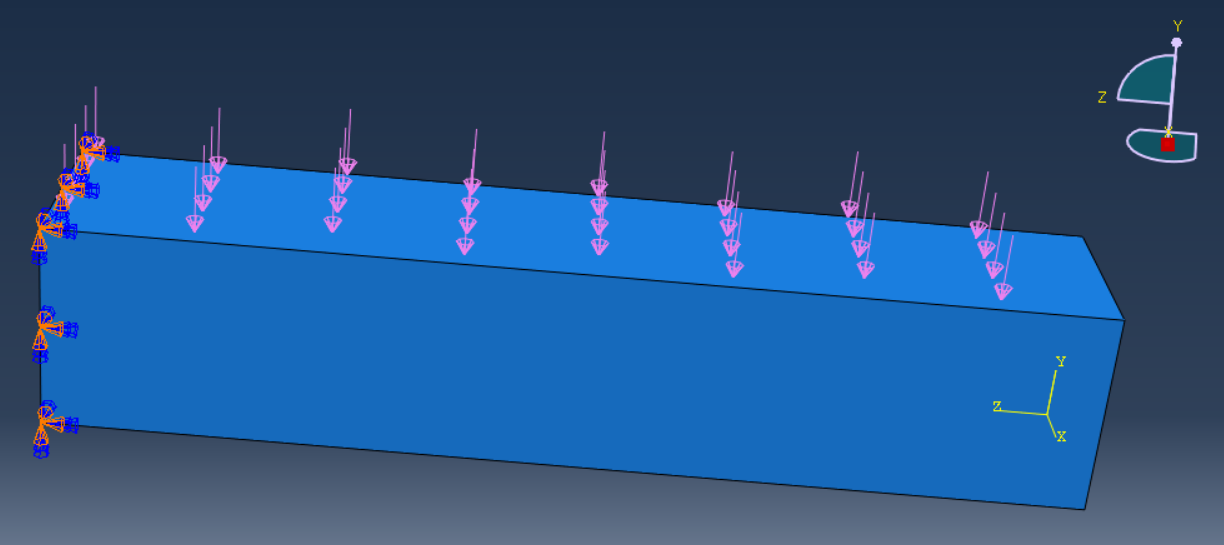
As an example, I’ll use a bending beam, since it is simple and mechanical engineers tend to like it 😊. The model is created in Abaqus/CAE. The beam is constrained on one side, while a pressure is applied to the top. Steel material properties are used.

Figure 1: Model set-up.

Various modifications to this model will be made using scripts.

Level 1: Exactly Repeat What Is Done Before

The simplest scripts to create, are those in which you exactly repeat something that is done before. This can be creating a material with specific properties (for a specific model name), creating a reference model, or doing postprocessing (when all names are the same). In those cases, we can simply record a macro. This can be done via file --> macro manager.

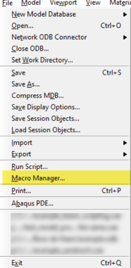
Figure 2: Accessing the Macro Manager.

Click on Create to make a new Macro, name it and choose whether it will be stored in the Home directory, or in the current work directory. Macros in the home directory are always accessible by the user and therefore more suitable for general purposes, macros in the work directory are only available in the current work directory and therefore more suitable for specific applications.

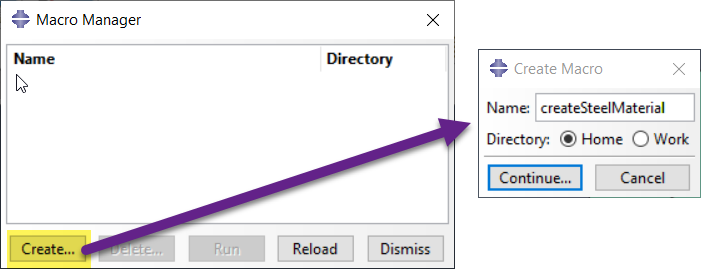
Figure 3: Macro Manager dialog box and create Macro dialog box. In this case there are no existing macros. Once they are created, they will be listed in the Macro Manager.

After clicking Continue make the (modification to) the model you are interested in and stop the recording. In this case we will create a material named steel with linear elastic properties. The createSteelMaterial macro appears in the Macro Manager. If we delete the current steel material model and run the macro, the material will be recreated. Similarly, if we open a new model database and run the macro, the material will be created.

Level 2: Modifying a Parameter

Macros that exactly reproduce what was done are often not very useful, because they are not generally applicable. In the previous example, with the steel material model, it would be nice if we can also use a different name, a different Young’s modulus and/or create the material in a different model. This can easily be done by slightly modifying the script. Let’s first take a look at the version created before, by opening it in Abaqus PDE (File --> Abaqus PDE). In Abaqus PDE select File --> Open and open abaqusMacros.py. This is in the home or the work directory, depending on where you chose to save the macro. In the code, we can recognize the model name, material name and material properties. These can all be given a name and value. By filling in different values for these parameters, the macro is more generally applicable. Save the modified version and reload and run it via the Macro Manager to try things out.

Figure 4: Original version of the macro, and an alternative version of the last section where model name, material name, Young’s modulus and Poisson’s ratio can easily be modified.

Aside: Asking for Inputs in a Dialog Box

To make things even more user friendly, it would be nice to have a dialog box pop up, that asks for these inputs. This can be used with the getInputs-function. An example is given in Figure 5.

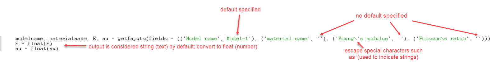
Figure 5: using getInputs to obtain a dialog box to request input

The resulting dialog box is shown in Figure 6.

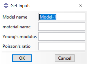
Figure 6: dialog box created using getInputs.

It is possible to make it more ‘fancy’ by adding a title etc; check the manual for the available options.

Level 3: Looping Over a Parameter

Often most benefit from scripting can be gained, if a slightly different version of a model is run multiple times. This means not modifying a parameter once, as we did before, but automatically filling in different values and rerunning the model each time. This parameter can be related to anything. It can be a material property, shell thickness, friction coefficient, … : anything that is described with a value in Abaqus/CAE. The script is typically just a few lines of code. We’ll show an example of rerunning a model with all stiffnesses from 150,000 MPa to 250,000 MPa, with increments of 25,000.

Obtain Code When Modifying Stiffness Manually

The easiest way to create the basis of the script is to record actions done in CAE in a macro or the .rpy file. In this case we record a macro when the stiffness is changed from 210,000 MPa to 190,000 MPa, a new job is created and the job is submitted. The exact values or names used do not matter, the main point is that we can see the command that is used to modify the stiffness and run the job.

Create Script to Repeat This Process

A new function is now added to abaqusMacros.py (Figure 7).

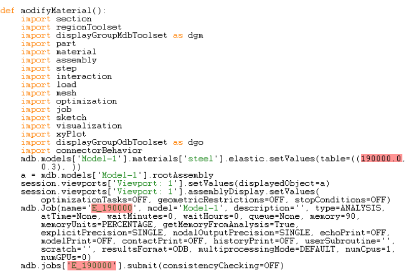
Figure 7: Recorded function when modifying the material properties, creating a job and running it.

We will now save the file under a different name, as a python script (.py extension). All macros except the one we are currently interested in, can be removed. Do leave the import statements at the top of the file. Remove the line containing ‘def’ and the indentation of the rest of the lines, so the code is no longer inside a function. We can then add the loop, a for-loop. In python, the syntax is as you can see in Figure 8. As you can see, there is no code to denote the end of the for-loop; this is clear because the indentation stops. Indentation is therefore very important in python.

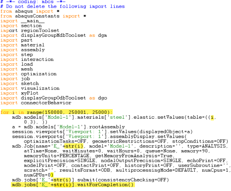
Figure 8: Code to run the model with stiffness from 150000 to 250000 and increments of 25000. It would be more elegant to define a name for the job, as was done in the previous section for the model name and material name. This version is shown since it has least modifications to the original code.

The variable i takes all variables in the range of 150,000 up to and excluding 250,001 with increments of 25,000. This variable is then used to specify the stiffness (first line in the loop) and to define the job name. With this method, the jobs all have a different and sensible name and data is not overwritten. In cases like this, you typically want to wait for the first job to complete before starting the second one. The function waitForCompletion does this. Only a few modifications to the macro therefore allow us to run a number of models without any further interference from the user.

Level 4: Changing a Location

In the example before a parameter was changed, something that is denoted with a value in Abaqus. We can use the same approach and modify the location of the load, rather than the stiffness of the material. This gives the function shown in Figure 9.

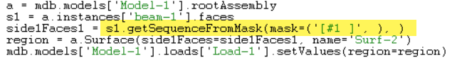
Figure 9: Excerpt from macro to change the surface on which the load is applied using default settings.

This script uses the command getSequenceFromMask to specify the faces on which the load is applied. This is very efficient, but difficult to interpret by humans.

You can choose how Abaqus defines geometry in replay files: via COORDINATE, INDEX or COMPRESSEDINDEX (the default). You can set this to coordinate by entering:

session.journalOptions.setValues(replayGeometry=COORDINATE)

in the command line interface. [The command line interface takes the same space as the message area, underneath the viewport. It is hidden by default, and can be accessed by clicking on the >>>-icon left of the message area.].

The macro resulting when replayGeometry is set to COORDINATE and the same steps are taken as before is shown in Figure 10.

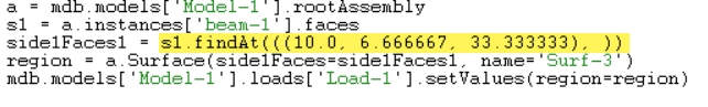
Figure 10: Excerpt from macro to change the surface on which the load is applied, using replayGeometry=COORDINATE

The code is now understood and modified more easily: if a different face is to be found, we can fill in the X- Y- and Z-coordinate of a point on this face. This point should not be shared with other faces.

Level 5: Changing the (Imported) Geometry

Up to now we have only changed part of the model and had relatively short scripts to achieve that. It is quite common to want to have the same simulation conditions on a different geometry. How can we achieve that?

If we would do it manually in Abaqus/CAE, then if the geometry is imported (which typically is the case) we need to redo the model set-up, such as reassigning sections and locations for boundary conditions and loads.

This means the script will be longer. In this example of a very simple model, when changing the geometry I already had 58 lines of code (excluding import statements), compared to at most 15 for the previous examples. For more complex models that have multiple parts, contact conditions etc., this will be a lot more. We will need to use the technique shown before (level 4) to locate relevant locations and make the script applicable to a new geometry as well. How difficult or easy that is to do, depends on the variations in geometry that are to be expected; more on that later (level 6).

It can be time consuming to create such a script. In some cases, especially when the geometry is simple such as in an axisymmetric model, it may then be more efficient to draw the geometry in Abaqus, in such a way that the dimensions that are to be varied are geometrical parameters. If these are modified, the surface ids will not change. Loads, boundary conditions or interactions applied to them are automatically updated. This requires more time during set-up of the initial model, but will allow you to make a geometric modification using the techniques mentioned under level 2, rather than level 4; which is much easier.

Level 6: Making a Script Generally Applicable

The most challenging aspect of creating a script is usually to make it generally applicable. The more we know about the model the script should be applied to, the easier it becomes to create the script. If we know the name of a material and the material model used, then changing a few parameters is straight forward. If we don’t know the type of material – it can be e.g. a hyperelastic rubber, or a plastic metal – then there are more choices to be incorporated in the script.

Especially geometric locations can be challenging to specify in a generally applicable manner. If we know there is a single face at a specified location, that is easy to script (as shown in level 4). If the surface we need consists of an unknown number of faces, and we do not know the exact location, it is more challenging. A definition of the faces must be provided. This is not always directly obvious and can be something such as the faces parallel to the xy-plane with the largest z-coordinate. Once this definition is deduced it must be converted to code, which can be a challenge in itself.

Conclusion

Getting started with python scripting does not have to be challenging: the difficulty depends on the problem at hand. A macro is typically a good starting point for a script. The closer the intended result is to the macro, the easier it will be to script. Changing parameters tends to be simple, changing geometry tends to be hard, especially if the script should be generally applicable and there is limited knowledge on the to be expected geometry.