In this blog post, we will be showcasing a fatigue assessment of a bicycle frame. This fatigue assessment will be against certain cyclic loading scenarios. Cyclic loading scenarios, typical for bicycle manufacturers, can include, pedaling forces, horizontal forces acting on the front fork and vertical load acting on the seat post.

For each of the aforementioned loading scenarios, an equivalent number of repeats until failure (log life) will be calculated and checked against the respectful number of repeats imposed by the used standard. The whole fatigue assessment workflow will incorporate different software.

At a first stage, Abaqus will be used, to setup the equivalent static load cases and boundary, corresponding to the different loading scenarios. The fea models used, will be linear (no material/geometrical/boundary nonlinearities were considered).

The results (*.odb format) of the Abaqus analyses, will be then given as input to fe-safe, wherein the fatigue assessment will be computed. The log life contours, will be mapped by fe-safe, to an *.odb format, for post processing in Abaqus.

Abaqus Model

As a first step, static linear perturbation steps will be run in Abaqus. Each step will correspond to a different loading scenario, with each respectful load magnitude being ramped up to 100%. The first load step will be the application of gravity and external loading steps will be run sequentially. Figure 1 below, shows the sequence of the various loading scenarios.

Figure 1: Sequence of loading scenarios.

Geometry, Mesh and Special Modelling Features

The bicycle frame geometry is shown below in Figure 2. The finite element model will mimic a typical bicycle frame test bench. Therefore, some add-ons have been created.

Figure 2: Geometry and modelling features.

In specific a steel front fork has been modelled. This will be used to apply the horizontal force and it has been modelled with beam elements. There is no interest on assessing the fork in terms of fatigue, that is why it has been modelled in a simplified manner.

The rear axle dropouts are connected to a beam connector. This beam connector mimics an add on, present on the test bench during testing. The boundary conditions on its bottom (at RP-4) are those that will vary per loading scenario.

Reference points RP-5, RP-6, have been placed at a certain distance from the frame’ s centerline and are connected to the bottom bracket (where the crankset and pedals are attached). Those RPs will be used for the application of the left and right pedal forces.

A beam connector has also been created and connected to the seat tube at the top of the frame. This connector mimics the seat post of the bicycle, upon which (on RP-7) the vertical load on seat post will be applied.

The mesh of the finalized assembly is shown in Figure 3. Beam elements have been used for the front fork. For the remaining geometry, first order reduced integration shells (S4Rs) have been used. A uniform thickness of 20 mm has been used for the bicycle frame, with the exception of the bottom sprocket which is 30 mm thick.

Figure 3: Mesh detail

Material Properties

In terms of material properties, a linear elastic material law was used. A steel material with elastic properties was assigned to the front fork. This component was not of interest for fatigue assessment. The remainder of the frame was made of aluminum alloy AL6061-T6. This alloy is probably the most extensively used material for aluminum bicycle frames, due to its high formability and easiness in welding/joining.

Since fatigue failure relates to cyclic loads, it is critical to use stabilized cyclic material properties, rather than monotonic ones (uniaxial). This is important, as stabilized properties vary from the uniaxial ones. In particular, cyclically loaded steel has the tendency to harden whereas aluminum softens.

Fe-safe software includes an extensive material library that is built in into the software. This includes many materials for which the fatigue life properties have been derived based on strain or stress-based fatigue tests. The user can search for a material based on its material class, code etc. A detail of this is shown in Figure 4.

Figure 4: fesafe built-in material database.

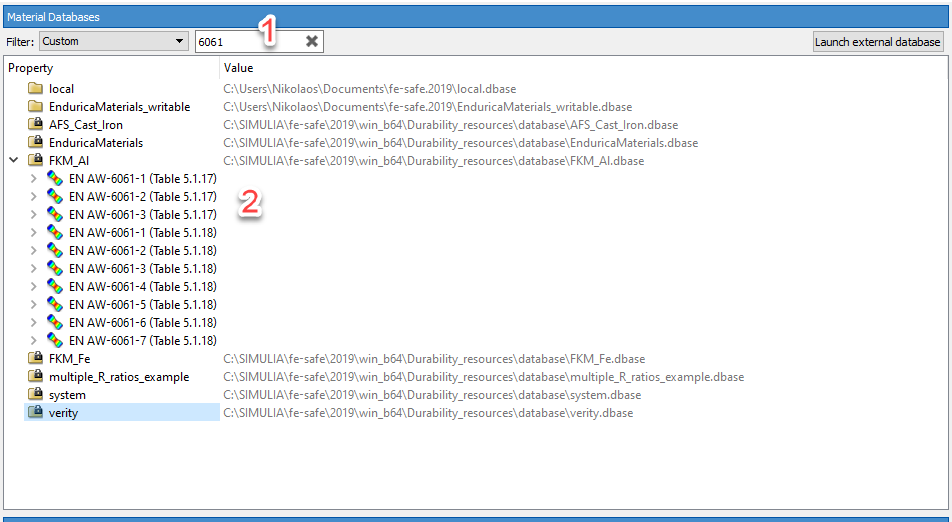
Since the material names shown in figure 4, do not entirely correspond to the material that we would like to use (T6 stands for tempering), we can also launch fe-safe’s external material database. A detail of the options and results of the external material database is shown in figure 5.

Figure 5: fesafe external material database.

When the specific material has been found, it needs to be exported from the external database and imported into fe-safe. This process is shown in figures 6 and 7.

Figure 6: fesafe import material database from external detail.

Figure 7: fesafe information of imported material database detail.

For the aluminum, a Young’s modulus of 69GPa and a Poisson’s ratio of 0.33 has been used in Abaqus (and fe-safe).

Loads and BCs

Figure 8 shows a screenshot from the various loads and boundary conditions. All forces (Except gravity) are concentrated loads, with magnitudes up to 1200 N.

Figure 8: Loads and BCs-Abaqus.

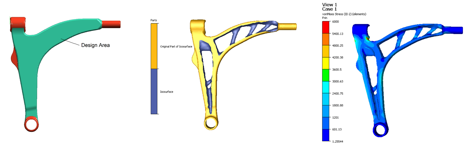
Abaqus Results

Figures 9 to 12, show the von Mises max envelope stresses in MPa (right hand side), per loading step, as well as the concentrated load magnitudes acting on the frame (left hand side).

Figures 9: Load case 1 Abaqus results.

Figures 10: Load case 2 Abaqus results.

Figures 11: Load case 3 Abaqus results.

Figures 12: Load case 4 Abaqus results.

fe-safe Model

Figure 13 shows the process of reading in the *.odb from Abaqus into fe-safe. It is quite straightforward to only read-in the stress datasets from each last increment (100% loading) in this case. Of course, there is the option to read-in elastic-plastic fea results, by reading in the respectful strains, but this could be meaningful in a case wherein a plasticity law was used in Abaqus.

Figure 13: Importing an fe model for fatigue assessment in fe-safe detail.

Table 1 shows the load magnitudes per load case, as well as the load ratios R. An R=0, means a loading cycle starting from 0 load up to 100% load and back to 0 (load on-load off). An R=-1 (known as fully reversed), means a loading cycle starting from 0 load up to 100% load and down to -100% load (fully reversed).

Table 1: Load case information.

For fatigue assessment, there is no need to implement the load ratios in the fea analysis with Abaqus. All we need to do in Abaqus, is run every step up to 100% load magnitude, and then the various load ratios can easily be assigned in fe-safe.

For the fatigue assessment, we will calculate the log life (Number of repeats) of the bicycle frame, per specific load case. For each load case, the effect of gravity will also be considered.

When the user has selected the stress datasets of interest (shown in Figure 13), the next window shows the element/section/material sets available, as those were defined in the fe model. This allows the user to quickly exclude element sets that are of no interest in fatigue. Fe-safe automatically creates an element set (“Element Surface” ), including all elements on the surface of a geometry, which are always the most critical for fatigue assessment (fatigue always initiates on the surface). A relevant detail is shown in figure 14.

Figure 14: Set groups detected and generated in fe-safe.

At the right-hand side in Figure 14, I have placed an element set (ALL_ELEMENTS_FATIGUE), that I created in Abaqus and will be assessed for fatigue. This set includes all the shell elements present in the bicycle frame. The element surface set of fe-safe includes a few more elements than my set, because it also contains the beam elements of the front fork, that are of no interest to us, for this fatigue study.

Figures 15 and 16 show details from the load case definitions in fe safe for load case 1 and 3 respectively (left pedal force and horizontal force front fork) as well as from the load ratios implementation. In figure 16, it is noted that R=-1. It is also noted that the effect due to gravity (dataset 1) is always present.

Figure 15: Load case 1 definition in fe-safe.

Figure 16: Load case 3 definition in fe-safe.

Figure 17 shows a detail from fe-safe’s analysis settings, where we have selected the element set of interest, for fatigue, and we have assigned AL6061 material to it. The default fatigue algorithm for AL6061 will be used, meaning the Brown miller strain-based algorithm with the Morrow mean stress correction (important to include as non-zero mean stress impacts fatigue life). Last but not least, the user can select a name for the *.odb that will include the log life contours and will be post processed in Abaqus.

Figure 17: fe-safe analysis settings.

fe-safe Results

Figures 18 to 21 below, show the generated log life contours as those were printed by fe-safe per load case. For the results presentation, a reversed rainbow spectrum has been used (red represents the lowest fatigue life).

In Figure 18, for the left pedal force load case, the lowest fatigue life will be on the frame tube connection to the bottom bracket. In specific, that frame location will endure 10^6.184=1,527,566 cycles of that specific loading before failing.

Figure 18: Load case 1 log life.

In Figure 19, for the right pedal force load case, the lowest fatigue life will be on the frame tube connection to the bottom bracket. In specific, that frame location will endure 10^5.796=625172 cycles of that specific loading before failing.

Figure 19: Load case 2 log life.

In Figure 20, for the horizontal fork force load case (fully reversing load), the lowest fatigue life will be on the head tube connection to the top and bottom tubes. In specific, that frame location will endure 10^5.25=177827 cycles of that specific loading before failing.

Figure 20: Load case 3 log life.

In Figure 21, for the seat post force load case, the loading magnitude and cycles induced, will result in an infinite fatigue life, as no fatigue failure will be caused due to that loading.

Figure 21: Load case 4 log life.

Concluding Remarks

As additional features to fe safe, all above load cases could have been combined in the same elastic block, in order to assess the frame’s fatigue life for the combined loading. Non elastic material properties and weld modelling can also be included, the effect of which can be considered for fatigue life assessment with fe-safe.