Metal Tube Hydroforming Process and Forming Limit Diagrams in Abaqus

In this blog post, we will be discussing about metal tube hydroforming with Abaqus. We will be using forming limit diagrams to create the material's strain envelope, for avoiding necking (rupture), a possible failure mode, in this type of metal forming process. This will be demonstrated in a hydroforming process simulation of a metal bellows joint.

Introduction

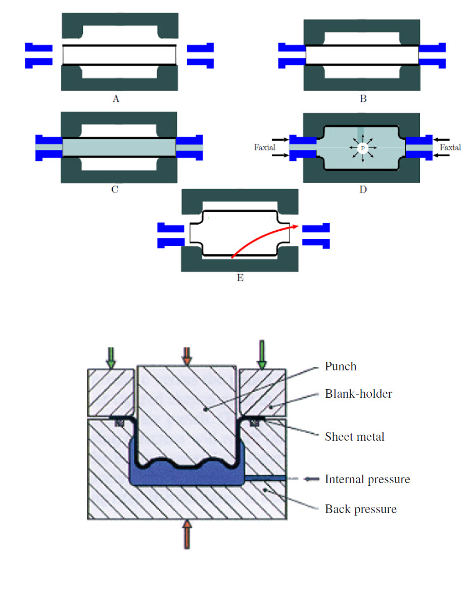
Metal hydroforming was introduced as an alternative to traditional metal forming processes, for mass production of work-pieces (tubes, blanks, preforms), primarily in the automotive and aeronautics industries.  Hydroforming utilizes fluid pressure primarily, to shape the work pieces.  There are two main categories in hydroforming, tube hydroforming and hydroforming of blanks. These are shown in Figure 1 below. 

Figure 1: tube hydroforming (top) and hydroforming of blanks (bottom). (Image courtesy of Wiley-material forming processes).

Another categorization of hydroforming processes would be as fixed die or moving die ones. Typically tube forming is considered as a moving die hydroforming process, as the work piece is formed under a combination of fluid pressure and axial compression, induced at the ends of the tube, which is termed as axial feed. Determining the optimal load path (combination between axial feed - fluid pressure) is critical for tube hydroforming  and is in many cases determined by trial and error, either with testing, or better yet with FEA.

Advantages

Advantages of the process over conventional ones include:

• reduced weight,
• uniform thickness of wall,
• reduction in tool cost (fewer components=less down time, more simplistic tool design),
• increased stiffness,
• reduced number of secondary operations,
• improved dimensional accuracy,
• less scrap.

Failure Modes

Typical failure modes in hydroforming include buckling, wrinkling and localized necking that leads to bursting/fracturing of the workpiece. For tube hydroforming, buckling and wrinkling (localized buckling) typically occur in the beginning of the forming process, and relate to excessive axial feed. Wrinkling can be corrected by slightly increasing the fluid pressure. Those modes are shown in Figure 2.

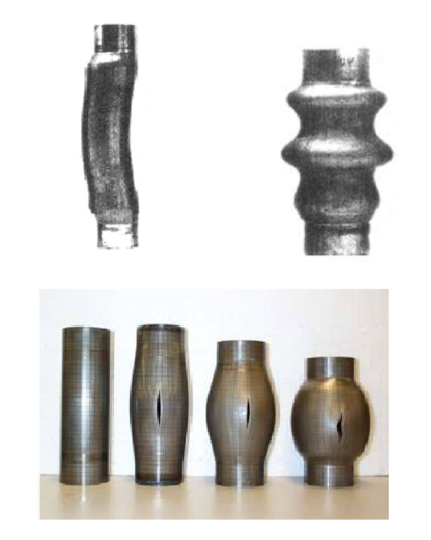
Figure 2: buckling (top left), wrinkling (top right) necking (bottom) failures in hydroforming. (Image courtesy of Wiley-material forming processes).

Tube bursting can occur due to necking. When necking initiates, strains become non uniform. Soon after, they localize, stiffness in that region is dramatically decreased and failure occurs. This type of failure occurs due to excessive fluid pressure. This is why finding an optimal pressure (e.g. load path) is really important in hydroforming and this mainly depends on material properties and the final geometry of the work piece.

Failure Criterion- Forming Limit Diagrams (FLD)

The Forming Limit Diagrams (FLD) are typically used, in metal forming processes, in order to assess, the formability of a work piece and avoid potential failure. Those are formed on the basis of major vs minor principal strain plots, under a biaxial strain state. As a newer advancement, Forming Limit Stress Diagrams (FLSD) have been used lately, as those are not sensitive to strain path changes.

The FLDs are attained experimentally with specific tests and are reliable predictors of fracture failure during the hydroforming process. To account for the uncertainties relating to the experimental data input, a safety margin on the Forming Limit Curve (FLC) of a specific material, is typically introduced.

The FLC curve of the high strength dual phase steel used in the example, is shown in Figure 3 below, in light blue color ("exp"). This was derived from testing. An exemplary design safety curve ("safety") is also shown, together with limit lines of certain material states for the specific steel.  Specific areas, where certain failure modes occur, are annotated in bold font in Figure 3 as well.

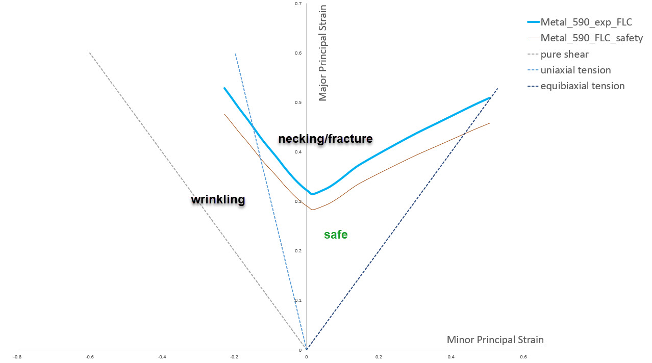
Figure 3: FLD of high strength steel.

Finite Element Model

A simulation of the hydroforming process of a 4 mm thick tube was investigated in Abaqus, to assess a specific high strength steel. The tube was hydroformed against a rigid die, to form a metal bellows joint. Abaqus Explicit was used (t=0.08 sec).

Model Details

Quarter symmetry was used in the model. A detail of the geometry (with rendered thickness) and loading is given in Figure 4 below. Shell elements were used for the steel pipe(grey white color)  and rigid shell elements (red color) for the die.

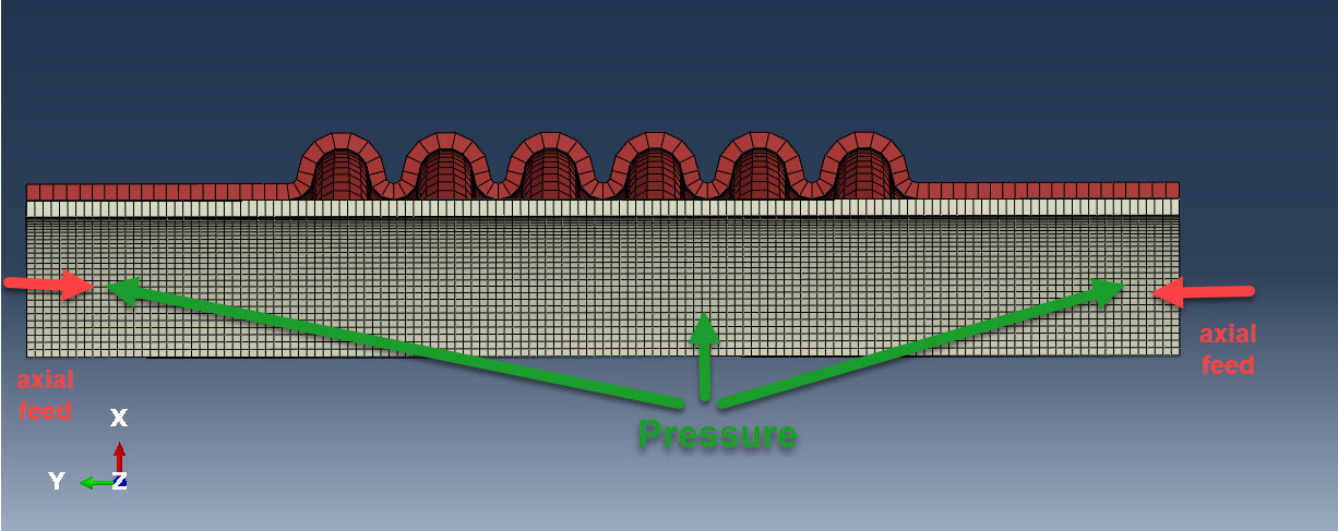
Figure 4: Rendered thickness Geometry, Mesh and Loading details.

Material Properties

In metal forming processes, anisotropic yielding is likely to occur. Isotropic elasticity was used. Hill's anisotropic yield law was used for plasticity in the fe model. The material true stress vs log plastic strain was given as input. For damage modeling, FLD damage (with the curve of Figure 3) was implemented, for predicting the fracture (more info here). The steel's stress vs total strain curve is given in Figure 5, together with a detail of the material tab in Abaqus.

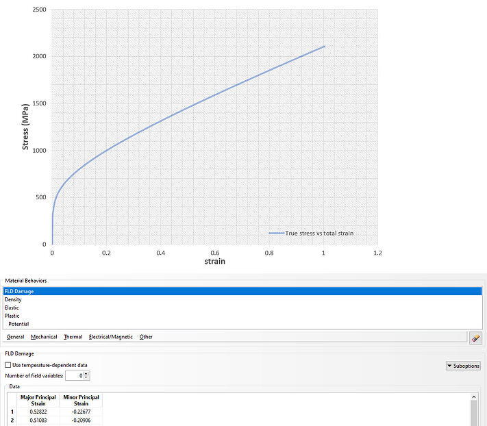
Figure 5: Material stress vs strain curve and material tab detail.

Loading

The loading input (Figure 4) during the hydroforming simulation, was implemented via an axial feed (synchronized at both ends-displacement control) under a certain amplitude, and a pressure load, under a certain amplitude, acting on the tube's surface. Those amplitudes are shown in Figure 6. This is called the loading path.

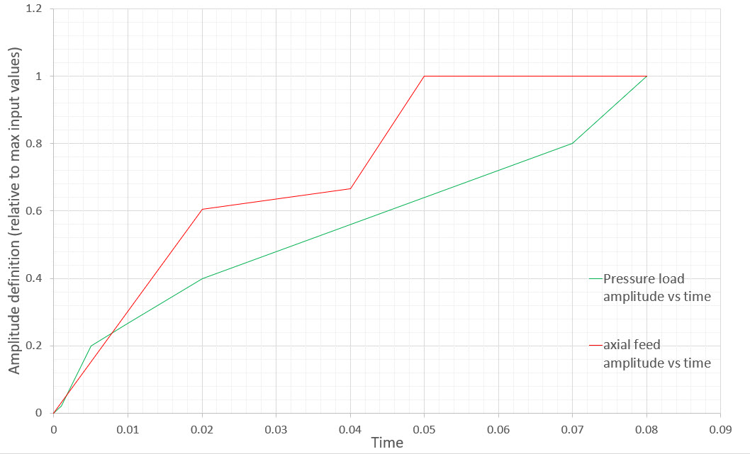
Figure 6: Chosen loading path for FE Analysis. 

Typically a larger increase in the pressure is desirable, in the beginning of the process, to stiffen up the material and avoid buckling/wrinkling failure due to compression from the axial feed (Figure 6).

Finding an optimum loading path, will result in a work piece with a better end quality. The chosen loading path here is a (relatively) random one.

Nowadays, FEA provides a feasible and accurate means of finding this optimum load path for metal forming processes.  Since this is an iterative process( finding this load path), FE Analyses are usually combined with optimization algorithms (using Isight for instance).

Results 

The results from the hydroforming simulation of the bellows are provided in images/videos below. 

Stress/Strain Results

Stress and strain levels and directionality (von Mises stress, max principal stress, max principal plastic strain) can provide insight on the material state and limits during the hydroforming process. Those measures can also help optimize the die geometry to help avoid hotspots on the work piece that can compromise its uniformity.

The respectful results (stresses in MPa) are given in the videos below.

Video 1: von Mises stress (MPa) on the bellows, during hydroforming.

Video 2: Max principal plastic strain on the bellows, during hydroforming.

Forming Limit Damage Criterion Results

Keeping track of the FLD damage (FLDCRT) will allow for insight on the formability limits of the material. This can help assess different materials and decide on the most appropriate one, for a certain hydroforming process or die shape.

The results of the FLD criterion are given below. As long as FLDCRT stays below one, the material point remains under the limit curve of Figure 3. For the bellows example, the material remained within forming limits, till 0.01 seconds prior to completion of the process.

At the end of the hydroforming simulation, failure was observed at the specimen (FLDCRT>1) at the location of the max plastic strain. A detail of the last two frames is given below, in Figure 7.

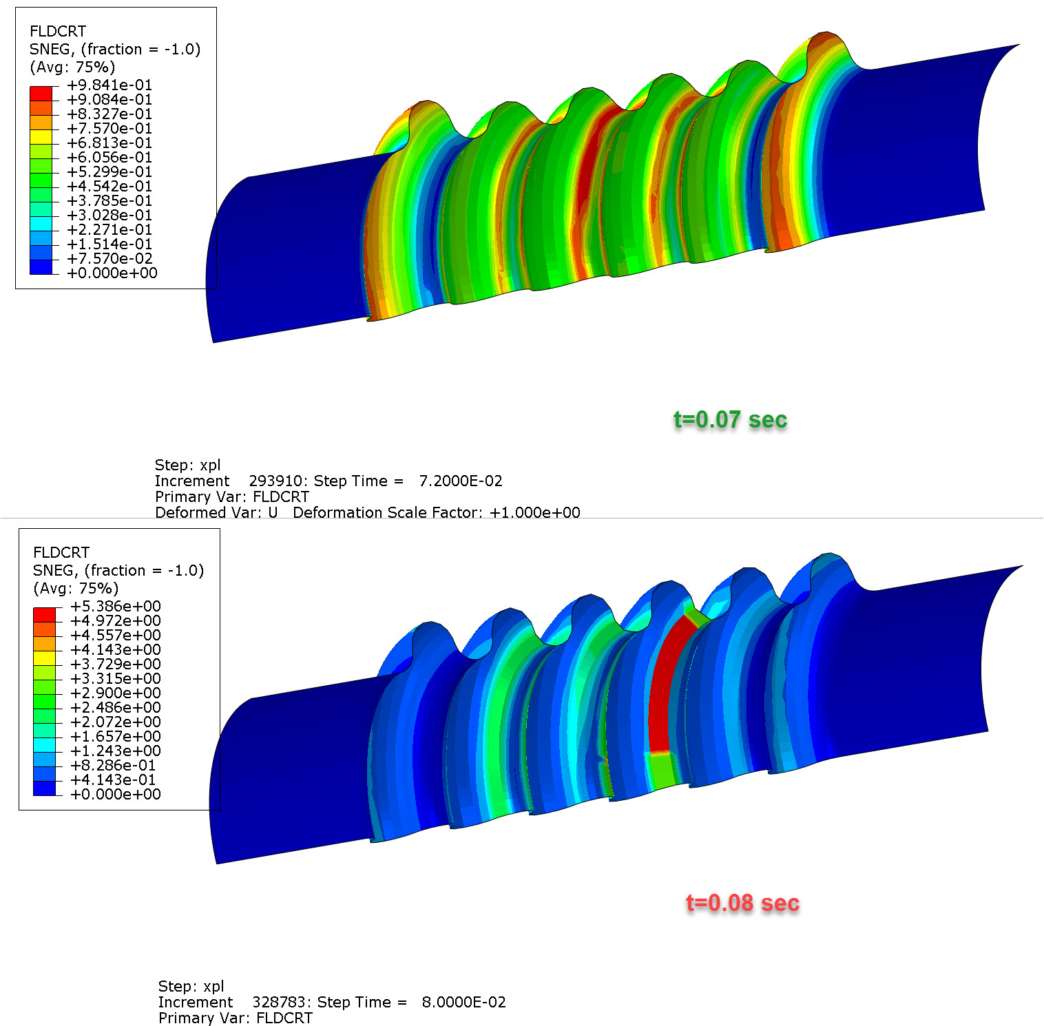
Figure 7: FLDCRT results (last two frames) for the bellows, during hydroforming.

The FLD criteria results for the hydroforming of the metal bellows, is given in the video below.

Video 3:FLD criterion on the bellows, during hydroforming.

Wall Thickness Results

The wall thickness results for the hydroforming of the metal bellows, is given in the video below.

Video 4: Wall thickness (mm) of the bellows, during hydroforming.

The initial tube thickness was 4 mm. Typically, in tube hydroforming a thickening of the tube's section is expected at the pipe ends, due to the compression from the axial feed. A detail from the final wall thickness (STH) of the bellows, is given in Figure 8 below (in mm).

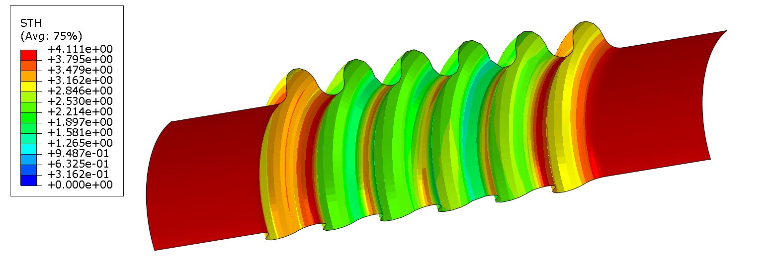
Figure 8: Final wall thickness of the bellows, at the end of hydroforming.

Inspection of the wall thickness uniformity at the end of the hydroforming process, can help assess the finished product's quality. A uniform wall thickness is desirable as much as possible.

Additionally the wall thickness, can help identify and improve the hydroforming process setup. By monitoring the wall thickness, an improvement of the loading path, e.g. the parameters of the amplitude curves of Figure 6 is possible.

This feature becomes particularly powerful, when coupled with optimization routines, that can modify certain input parameters (loading path, process time) in order to stay within a percentage of thickness reduction in the work piece.

Discussion

In the section above, results from a hydroforming simulation of a bellows were presented. Hydroforming processes have become quite popular due to their aforementioned advantages over traditional forming processes.

Additionally due to the new C02 emission regulations, dictating weight reduction of components, while structural requirements stay fixed, hydroforming is expected to be used more extensively in the coming years. The uncertainty in the parameters relating to the hydroforming process, makes the use of computer models quite appealing, for simulating/optimizing hydroforming. 

Some of the benefits of simulating hydroforming are the following:

• possibility to accurately predict the actual stresses/strains developed during the process,
• possibility to implement FLD damage to assess the formability of a material and to even stay under a certain FLD limit percentage,
• possibility to investigate die-workpiece frictional characteristics and to modify those in order to achieve a specific bulge height for the bellows,
• possibility to minimize the % of FLD with an optimization routine (Isight or similar software can be used),
• possibility to assess different materials for a certain hydroforming process and/or work piece geometry,
• possibility to optimize the specimen geometry to get rid of stress hotspots,
• possibility to optimize the loading path parameters of the hydroforming process to achieve maximum wall thickness uniformity or to stay within a certain range of thickness reduction (Isight or similar software can be used).