Modeling Bolted Connections with Abaqus FEA

In this blog post, we will be discussing about the different methods in modeling bolted connections with Abaqus FEA. At the last section of the post,we will be showcasing a bolted connection, incorporating a pretensioned bolt. Flanged connections are used extensively in most engineering disciplines. They provide a way of interconnecting  various (metallic, plastic etc.) components and their design is often critical for the strength of various components (e.g. bolt strength) and sealing of the assembly. 

Bolt Modeling

With respect to the modeling of bolts in  a flanged connection, various modeling strategies are available, based on the level of accuracy required (simplest to most accurate):

Simplest Method for Modeling Bolts

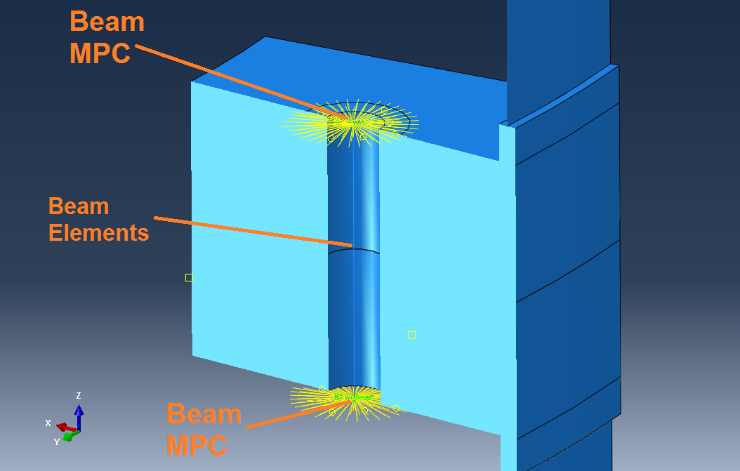
The simplest method for modeling bolts can be seen in Figure 1. In this figure the circular beam profile, corresponding to the bolt shank, is not shown to assist visualization.

Figure 1: Modeling bolts with beam elements and Multi Point Constraints (MPCs).

In the method shown in figure 1, two MPCs have been created, in order to connect each end point of the beam (the beam elements represent the bolt's shank), to the joint members.

As the control point, each of the beam's end points is first selected. As a slave region to be selected for the MPCs, the user can select a circular area on each of the flange faces (or create those partitions) , corresponding to the dimensions of the nut,grover or bolt head that fits to the given bolt dimension (use metric bolt sizing tables to find this information).The total number of MPCs created should be two ( one per connection to the each of the flange faces).

The bolt's shank, represented by beam elements with this approach, should have a circular beam profile. 

As an alternative approach to modeling the bolt shank with this method, connector elements can be used instead of beam elements.

This method, does not allow for contact interactions between the bolt's end features (such as nuts or heads), and the joint members (flange faces).

More Accurate Method for Modeling Bolts

As a second approach for modeling bolted connections by adding a bit more complexity and allowing for contact definitions between bolts and joint members,  a combination of shell elements and connectors can be used. This is shown in Figure 2.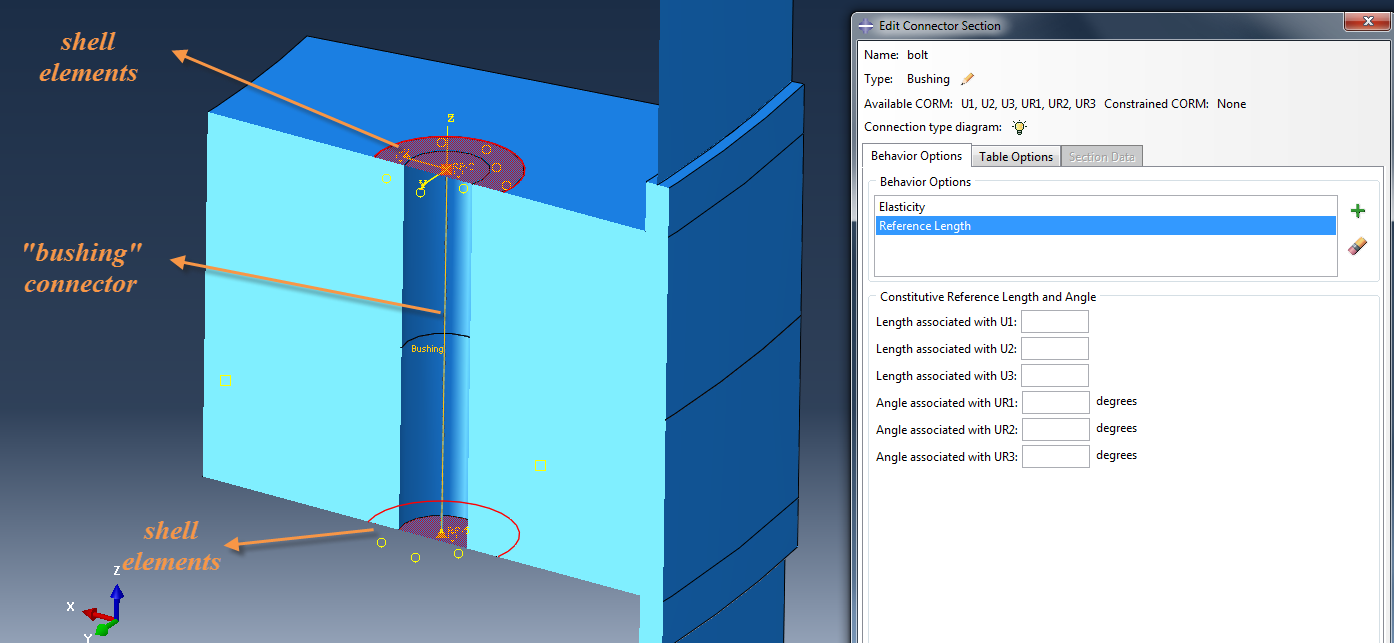

Figure 2: Modeling bolts with connector and shell elements.

In the method shown in figure 2, two planar circular sections have been created and discretized with shell elements.These shells represent the end geometry of a bolt.

The section dimensions of each shell, should correspond to the dimensions of the component modeled (e.g. the height of the bolt head, the height of the nut or grover etc.). 

In this method, the bolt's shank will be modeled by creating a connector of the "bushing" type. This can be done via the Abaqus connector builder, that is quite straight-forward and user friendly.

Two RPs in total  should be created at the centers of each planar shell (shown in figure 2). These RPs should then be used in order to create a wire feature, to be subsequently assigned with the connector section. This connector section should then be assigned with relevant properties, as shown in Figure 2.

Since the RPs belong to each of the shells, there is no further need for connecting the bolt's shank to the bolt's ends.

The user can then create ties between the shell surfaces and surfaces of the joint members (flange faces connected to bolts). Or better yet, contact interactions can be created instead of ties, as this method allows for this, unlike the method that was previously explained.

As an alternative suggestion with this method, beam elements can still be used instead of connectors, for the bolt's shank. Alternatively, for modeling the end geometry of a bolt, solid elements can be used instead of shell elements.

Most Accurate Method for Modeling Bolts (Solid Elements)

As a 3rd and most accurate method for modeling bolted connections, the bolt's entire geometry (including end components such as nuts and grovers) can be modeled with solid elements. This method allows for contact interactions between all involved components as closely to reality. This method is shown in Figure 3.

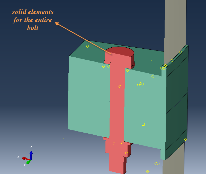
Figure 3: Modeling bolts with solid elements.

For this approach, modeling takes place more quickly, if bolt shank and all related components (bolt heads, nuts etc.) are modeled as one part. Of course this is not mandatory and proper ties can be assigned for connecting all components of the bolt "assembly" . 

As was mentioned, this approach allows for assigning contact interactions, between all relevant components/parts that come into contact in a bolted connection. Relevant candidate contact pairs are given in figure 4 below.

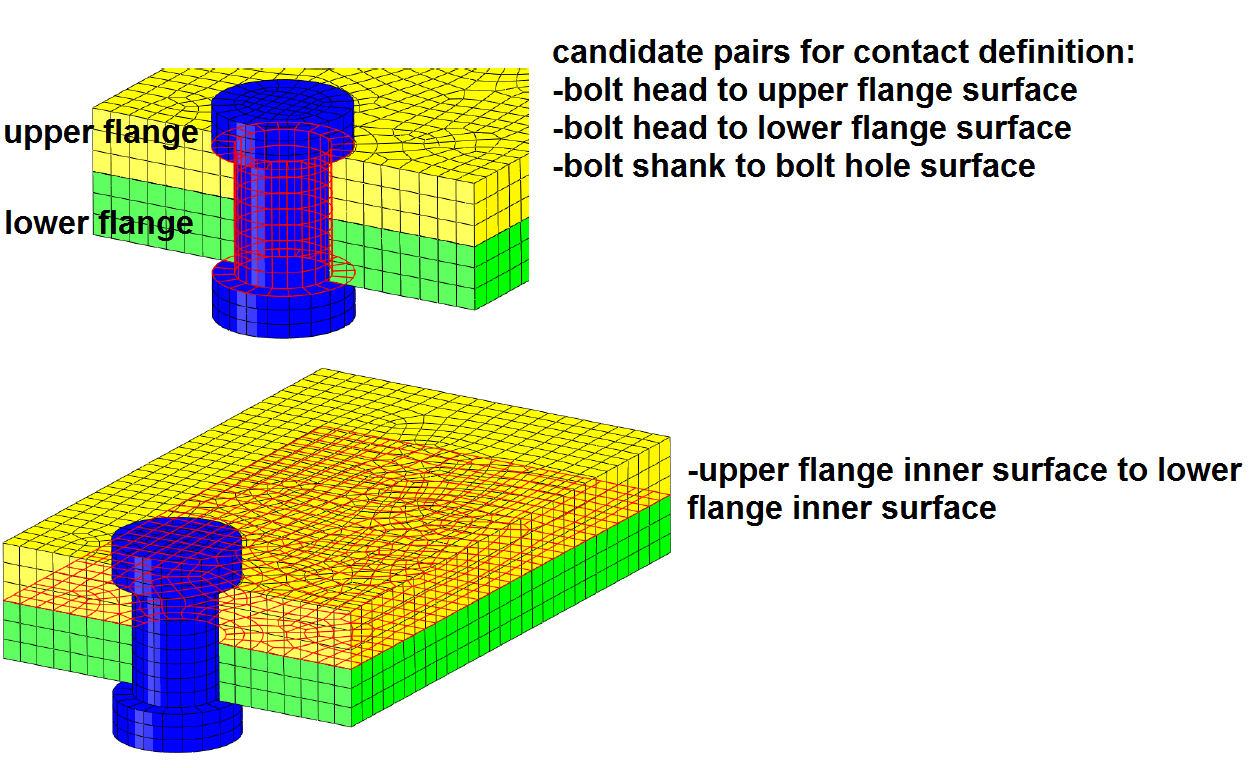
Figure 4: Candidate contact pairs for bolted connection modeling.

With respect to the candidate pairs as shown above, the selection of those depends on the level of detail needed in combination with the end goal of an analysis.

If possible, tie components in order to minimise computing needs.

However modelling contact can be necessary if the loads acting upon the bolted connection, can cause:

-Separation of faces

-Slippage (of interest in shear slip-resistant joints)

In a situation where only the potential gap formation between flanges under external loading is of interest, the bolt heads can be directly tied on the respective flange surfaces. Then the only contact definition needed, is a contact pair between the inner surfaces of the flanges, in order to properly track the remaining contact pressure and potential gaps.

This last case will be demonstrated at the last section of this blog post as an exemplary case.

Pretension Options

For bolt pretensioning in Abaqus, the preload can be applied as a force or as a reduction in length. A detail of both options is given in Figure 5. 

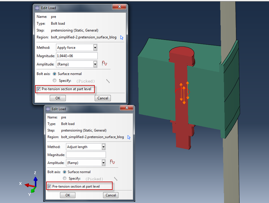
Figure 5: Methods for applying pretension on solid bolt.

Feel free to try out pre-tension at part level. This feature is particularly useful in full 3d models, where a pretension load must be applied in many bolt instances, all of which are derived from the same part. Pretension at part level, allow the direct application of pretension loads in all bolt instances, by only creating a single bolt load definition in the load module. This feature is quite useful since in the past, applying pretension loads in large number of bolts could only be realised via scripting.

To aid convergence, occasionaly it is better to apply a length reduction initially and then change to the required force in the next step.

Remember to switch the bolt load to--> "fix at current length", for subsequent loading steps, after the full pretension has been applied. Otherwise Abaqus will continue to apply pretension force, which is not correct.

Exemplary Case (3d Sector Model)

A 3d sector of a steel flanged connection will be shown as a relevant example.

This sector comprises of:

two flange members, interconnected by a pretensioned bolt. Additionally after the bolt has been pretensioned (using the force method), the connection is put under external loading, in terms of a bending moment acting on the connection's wall (via an RP).

Joint members and bolt have been modeled with solid C3D8R elements. Remember to use these elements in bending dominated problems as first order full integration elements lock in shear. Also try to use at least 4 C3D8R elements on the thickness direction in order to avoid hourglassing, inherent to those reduced integration elements.

The wall, has been modeled with shell S4R elements. The bending moment is applied on a remote RP, that is connected with the upper wall, through a kinematic coupling. The same approach has been used in order to fully fix the lower part of the wall of the bolted connection. A remote RP has been first kinematically coupled to the lower wall and all 6 dofs on that RP have been constrained.

Since the walls, representing a shell structure, are connected with the solid flanges, two Shell to Solid couplings have been created in total, to impose the proper connections between the different element types.

All the aforementioned modeling features are shown in Figure 6.

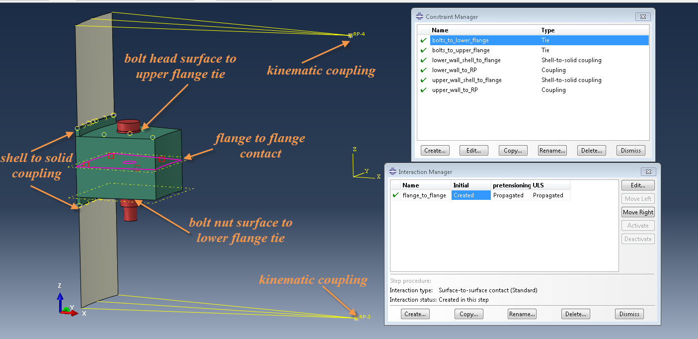
 Figure 6: Modeling features of exemplary case.

 The only contact definition, is for the inner flange surfaces (flange to flange contact) in this example. A typical hard to hard contact (normal behavior) together with a friction coefficient of μ=0.5 (tangential behavior-typical value for steel to steel interactions) have been assigned as the interaction property.

Also the faces of the bolt end components (e.g. bolt head and nut) have been directly tied with the exterior flange surfaces, in order to properly impose the bolt pretensioning.

Alternatively, In a more detailed analysis, those faces could have been assigned with contact interaction with the respective exterior flange faces. Also a tie  or a contact pair between the bolt shank and bolt hole could have been assigned based on focus of the analysis.

For this example , the main analysis focus, is the resulting contact pressure contour, after the external loading has been applied. A detail of the contact pressure (CPRESS output variable) on one of the flange members is given in Figure 7 for both the end of the pretensioning step and the external loading step. This allows for a direct comparison of the contact pressure contours, after bolt pretension and after external loading has been applied. 

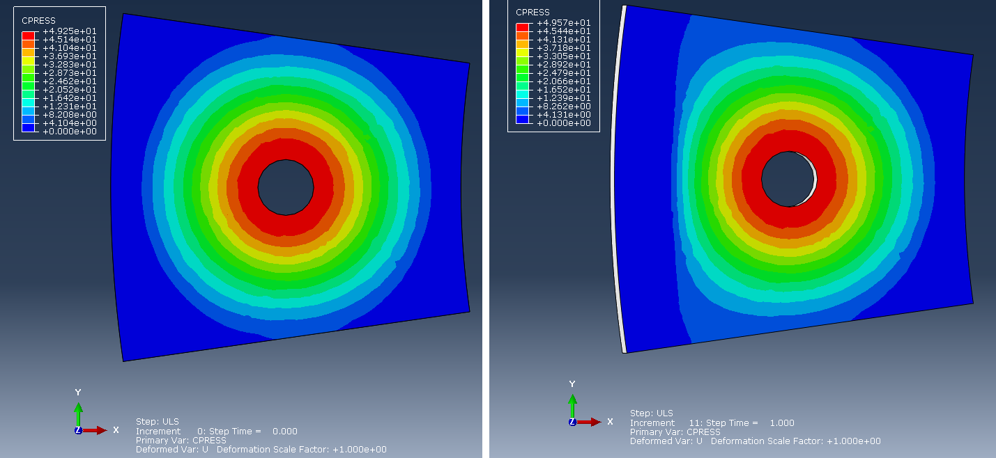
Figure 7: Contact pressure contour after bolt pretensioning (left) and after external loading (right).

An output variable that is particularly useful, when tracking potential gaps occuring at flanges under external loads, is the COPEN variable. A relevant detail is given in figure 8.  The minimum contour limit has been set to zero. What is colored as black, then indicates a positive (existing) contact pressure. Plainly said, the COPEN variable can be considered as the inverse of the CPRESS variable.

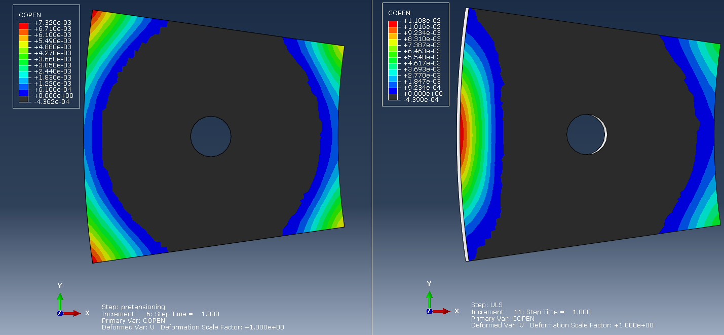
Figure 8: Contact opening contour after bolt pretensioning (left) and after external loading (right).

 A video of the overall flange motion and displacement (in millimeters) is given below.