Modelling a Composite Flanged Tube Including Loading With Abaqus/CAE

In this blog, we will be providing information on the modelling of laminated composites with Abaqus. Modelling will be done using the composite layup tool, and material orientations will also be assigned.

Those modelling features will be demonstrated with a relevant example case of a composite flanged tube under loading. The tube will be subjected to thermal and radial pressure loading.

Introduction

Stress and deformation analysis of laminated composites can be done at different modeling scales.

Those are shown in figure 1.

Figure 1: Different scales of laminated composite modelling (a:microscale,b:mesoscale,c:macroscale).

When a great level of detail is necessary, the strains and stresses can be calculated at the constituent level, meaning the fiber and matrix separately. It is necessary on this micromechanics scale modeling, to describe the microstructure including the fiber shape and distribution as well as the material properties of the constituents.

In most cases, strains and stresses must be calculated for every lamina in the laminate structure. Then the laminate stacking sequence must be given as input. This information will include the elastic properties of each lamina, its respectful thickness and fiber orientation. This is the mesoscale level of modeling.

In the crudest form of modeling, the composite is modelled as a homogeneous equivalent material. If the laminate is analysed as a homogeneous equivalent shell, the stress distribution within the laminate cannot be obtained. This approach becomes meaningful when displacements, buckling modes or frequency analysis is the end goal of the modelling.

Generally speaking, the micromechanics approach is usually avoided in most cases. Instead either properties of the basic unidirectional lamina or of the whole laminate can be defined experimentally.

The laminate properties in Abaqus, are specified in two ways:

-by the constitutive matrices A,B,D,H or

-by specifying the laminate stacking sequence and properties of every lamina.

When the A,B,D,H approach is used, the shell element cannot distinguish between different laminas (and therefore stress distributions within the laminate cannot be obtained).

Geometry and Mesh

In the blog example we will be using the laminate stacking sequence approach, using 1^st order reduced integration conventional thick S4R shell elements.The geometry and respective mesh of the blog’s example are shown in figure 2.

Figure 2: Geometry and Mesh of flanged tube example.

Loads and BCs

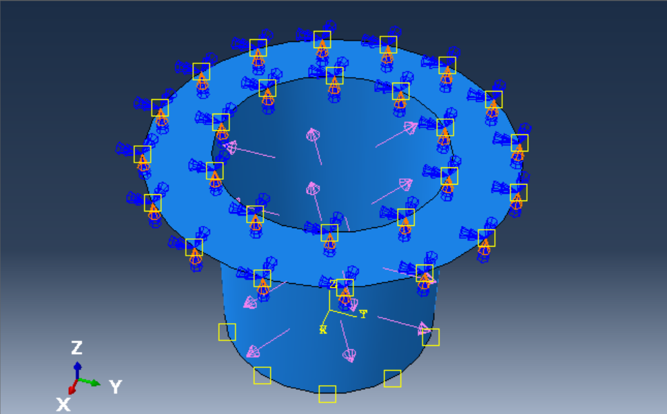
The loads and BCs are given in Figure 3.

A thermal load of 150 degrees and a radial pressure are acting on the flanged tube. The flange(top) region of the tube, is simply supported (U3=0).

Figure 3: Loads and boundary conditions of flanged tube example.

Material Modeling

Material Properties 

Under plane stress conditions (since shell elements are used), only the values of E1,E2,ν12,G12,G13,G23 need to be specified. The part will comprise from a unidirectional carbon/epoxy composite material, the properties of which are given below in figure 4, in units of MPa. In the same figure, the orthotropic coefficients of thermal expansion are also given. The respective material directionalities will be assigned according to the material direction provided in the composite lay-up window.

Figure 4: Material properties of flanged tube example

This material will be arranged in [0/45/-45] configuration for the entirety of the flanged tube geometry, for both the cylindrical part of the tube as well as for the flange on top.

Material Orientation Example

Figure 5, shows an example of the composite lay-up window in abaqus. It can be seen that both plies, vertical tape 1 and vertical tape 2, define their orientation by using the default layup orientation (CSYS:Layup). The fibers of vertical tape 2 have a 90 degrees rotation with respect to the 1-direction of the Layup orientation coordinate system.

The various composite lay-up window settings are explained next.

Figure 5: Exemplary composite layup from Abaqus documentation.

Layup Orientation

The layup orientation defines the base or reference orientation of all the plies in the layup. In conventional shell layups, Abaqus projects the specified orientation onto the surface of the shell, aligning the direction of the layup orientation that you choose with the shell normal.

Abaqus/CAE provides several options for defining the layup orientation. More information on those can be found in the documentation link (abaqus documentation link).

Ply Orientation

The ply orientation defines the relative orientation of each ply.

Coordinate system

Abaqus/CAE provides the following options for defining the coordinate system of the ply:

• Layup: By default, the coordinate system of the ply is the same as the coordinate system of the layup.
• CSYS: You can create and select a datum coordinate system that defines the coordinate system of the ply. If you choose to use a coordinate system for a ply, it overrides the layup orientation for that ply.You can also select the axis of the coordinate system that defines the normal direction of the ply. The axis that you choose appears as the last digit in the CSYS column in the layup table. For example, Datum csys1.3 indicates that you chose Datum csys-1 to define the coordinate system of the ply, and you chose the 3-axis to define the normal.
  

  For the flanged tube, in order to facilitate the fiber directions, a user defined cylindrical coordinate system will be created. This is indicated in Figure 6 by the orange arrow.

  The axes correspondence to the cartesian rectangular coordinate system is X:R,Y:T,Z:Z.

  For the cylindrical region of the flanged tube, the reference orientation of the plies, will be the symmetry axis of the cylinder (Z-axis). Figure 6 shows the composite lay-up settings assigned for the cylindrical region. For all the plies, the normal has been defined as axis 2 (T) of the user CS. This will constitute therefore, direction 3 (normal n: red arrow), and the reference orientation (Ref1) will be assigned accordingly. The photo shows the orientation of Ply-1, that has no additional rotation angle (0) with respect to the reference orientation. The resulting fiber orientation of ply-1 is indicated by the light blue 1-axis.

  

Figure 6: Composite layup settings for the cylindrical region.

Figure 7 shows the composite lay-up settings assigned for the flange(top) region. For all the plies, the normal has been defined as axis 3 (Z) of the user CS. This will constitute therefore, direction 3 (normal n:red arrow), and the reference orientation (Ref1) will be assigned accordingly. In this region, the reference orientation of the fibers will be the radial one. The photo shows the orientation of Ply-2, that has an additional rotation of 45 degrees with respect to the reference orientation. The resulting fiber orientation of ply-2 is indicated by the light blue 1-axis.

Figure 7: Composite layup settings for the flanged region.

Figure 8, shows the ply stack plot for the flanged region of the tube. This stack plot, can provide a visual verification of the assigned properties of each ply (thickness and fiber orientation). 

Note that in the stack plot of Figure 8, the reference surface for the shell is also shown. You need to make sure that for the flange region in this example, the reference surface is set to bottom (instead of midsurface), in order to avoid material overlap between the two regions(flanged and cylindrical).

Results Visualisation

Figures 9, 10 and 11, show the stress(S11) in MPa along the fiber directions, for ply-1 (0 degrees fiber), ply-2(45 degrees fiber) and ply-3 (-45 degress fiber) respectively. On the right hand side of those photos, the fiber orientation (indicated by the light blue line) is also shown. 

Figure 9: fiber stress on middle section point location, for the lowermost (ply-1) ply (left) and respective fiber orientation(right).

Figure 10: Fiber stress on middle section point location, for the middle (ply-2) ply (left) and respective fiber  orientation(right).

Figure 11: Fiber stress on middle section point location, for the uppermost (ply-3) ply (left) and respective fiber orientation(right).

The results visualization of the composite flanged tube is also shown in the below video.