Non-Linear Optimization of a Connecting Lug with Tosca Structure

Introduction

Tosca is part of the Abaqus Unified FEA product suite. It can be used for non-parametric optimization. It offers both structural (Tosca Structure) and fluid (Tosca Fluid) optimization capabilities.

In this blog, we will focus on the former and present examples of advanced structural optimization. Tosca has its own GUI named Tosca Structure GUI, but it is also implemented with almost all the features in the Optimization module in Abaqus. The following optimization types are available:

• topology - modifies the whole volume,
• shape - modifies the surface,
• sizing - modifies shell and beam thicknesses,
• bead - creates bead patterns for shell structures.

One of the biggest advantages of Tosca Structure is its capability to solve optimization problems with all three types of non-linearities:

• material,
• geometrical,
• boundary (mainly contact).

This blog presents a simple example of a lug. This case is well-known from Abaqus documentation (Getting Started with Abaqus/CAE guide) and intro courses, but here we won’t focus on its mechanical simulation but on the possibility to optimize its geometry. We will cover two different cases:

• sizing (thickness) optimization of a shell model of the lug,
• topology optimization of a solid model of the lug.

Both cases will be solved with both linear (tie constraint) and non-linear (contact) approaches, showing completely different results of the optimization. (Non)-linearity here is understood as boundary (non)-linearity because geometrical non-linearity was included in all the runs but had no significant impact on the results here.

Sizing Optimization

The first case was the sizing optimization of a shell representation of the lug. The figure below (Fig. 1) shows the mesh used in this example. In addition to the lug (with an initial thickness of 0.003 m - to be changed by the optimization algorithm), a discrete rigid pin was included in the model.

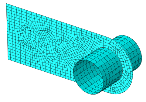
Fig. 1. Shell mesh of the lug and pin assembly.

The lug was fixed on one end, and the pin was pulled with a force of 12500 N to stretch the lug. Boundary conditions and loads are shown below (Fig. 2).

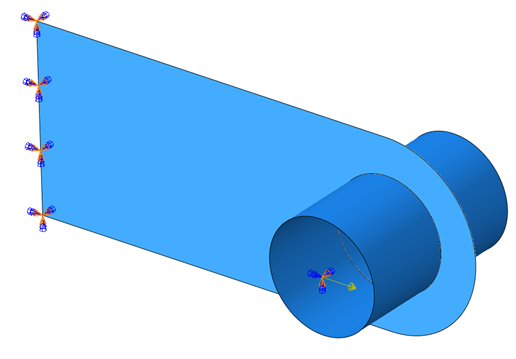
Fig. 2. Boundary conditions and loads in the lug and pin model.

Linear elastic material was used, a general static step was defined, and no other special features were utilized in this analysis. Thus, we can proceed with the setup of the optimization case. The first step was to define the optimization task. Sizing optimization was selected, and load regions were chosen to be frozen. Two design responses were defined: Mises stress in the whole lug and volume of the lug. They were used in the objective function and constraint definitions:

• objective function: minimize volume,
• constraint: stress less or equal to 2e8 Pa.

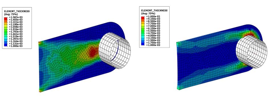
Fig. 3. Result of the linear (left) and non-linear (right) sizing optimization approach with horizontal load - shell thickness visualization and contour plot.

Additional runs were done with a different load case - vertical downward force of 5000 N. The rest of the setup (apart from the pin boundary conditions that had to be adjusted for the new load case) was the same. The results below are for the linear and non-linear approach (Fig. 4).

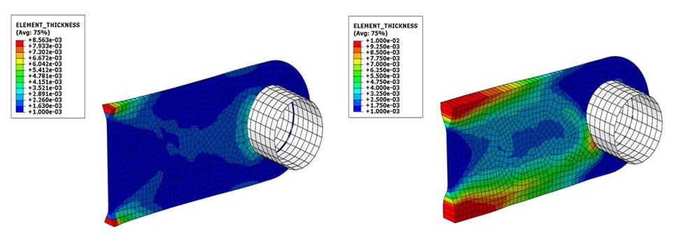
Fig. 4. Result of the linear (left) and non-linear (right) sizing optimization approach with vertical load - shell thickness visualization and contour plot.

Topology Optimization

The second case was topology optimization of the lug. The solid model known from Abaqus documentation and courses was utilized, and only the pin was added. The mesh is shown below (Fig. 5).

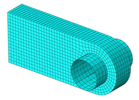
Fig. 5. Solid mesh of the lug and pin assembly.

The boundary conditions were the same as in the shell model, and only horizontal load (the same value as before) was used to show a large difference in the results of the linear and non-linear optimization cases. The topology optimization task was defined with boundary condition regions frozen. Design responses included strain energy and volume. They were used in the objective function and constraint definitions:

• objective function: minimize strain energy (= minimize compliance = maximize stiffness).
• constraint: volume less or equal to 40% of the initial volume.

Also, geometric restrictions were defined to enforce planar symmetry with respect to the horizontal symmetry plane of the lug.

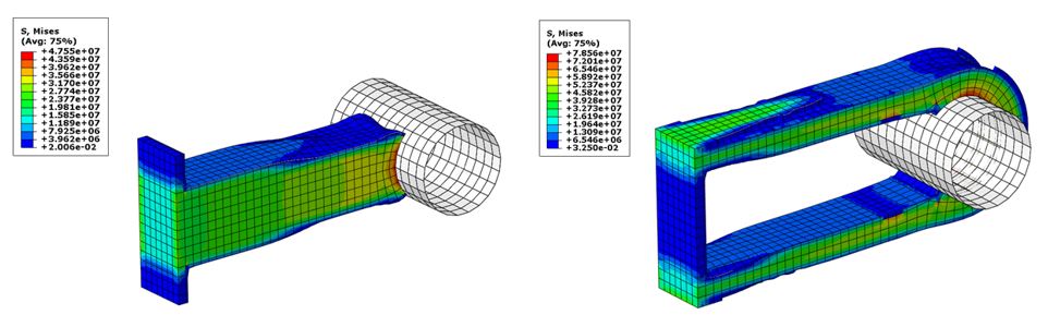
The figure below (Fig. 6) shows the results of the linear run with tie constraints and the non-linear run with contact.

Fig. 6. Result of the linear (left) and non-linear (right) topology optimization approach - Mises stress contour plot.

Summary

The results of the first case (sizing optimization) show that the optimized thickness distribution has a significant dependence on the approach being used. It is even more visible in the vertical load case.

The results of the second case (topology optimization) are completely different when contact is used instead of a tie constraint. As can be expected, the result of the run with tie constraint is caused by the fact that this constraint forms a complete bond (no sliding and separation) between the whole surfaces. The result of the run with contact accounts for the fact that contact (normally) is a compression-only constraint, and tension is not resisted.

As shown in this blog, Tosca can easily handle optimization cases with non-linearities, including non-linear contact conditions. The difference in the results is so significant that the shapes obtained for linear approach can be considered useless and unphysical, meaning that models like this should always be optimized with non-linear contact included.

You could also extend this case to show the influence of plasticity on the optimization results, but the goal here was to cover boundary (contact) non-linearity. Tosca, with its state-of-the-art non-linear optimization approach, is a perfect choice for problems of this kind.