Beyond Subroutines in Abaqus/Standard

Let’s explore how to use new keywords to streamline this process in Abaqus/Standard, and we’ll come back to Abaqus/Explicit in a future discussion.

You might be asking yourself, “What type of problem could benefit from the solver’s ability to independently terminate a step or the entire analysis?”

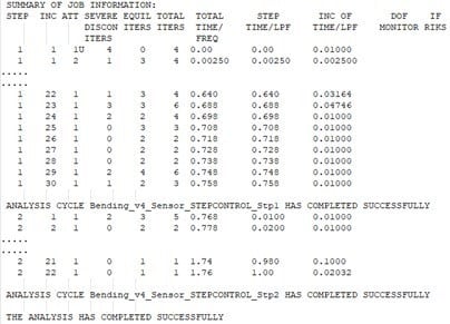
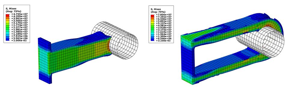
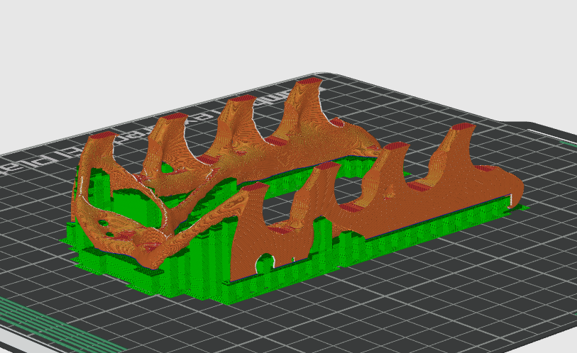
Well, let’s take the model below as an example. It’s a simplified representation of a 3-point bend test, used during TECHNIA Simulation training sessions to examine the impact of different non-linearities on the best simulation strategy to employ. All elements are present: contact (with friction), geometric non-linearity, and, crucially for this discussion, plasticity, which is simplified to a bi-linear elastic-plastic response.

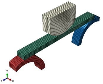
The simulation comprises two static steps. Mechanically, the two lower rollers are fixed, and the upper crosshead is moved downward to bend the bar and induce plastic deformation during the first step of the simulation. In the second step, the crosshead is returned to its original position to observe the elastic springback and residual deformation of the part.

To enhance convergence in the loading step (where the residual forces in the bar are balanced solely by the contact forces on both its top and bottom faces) and, importantly, to efficiently return the crosshead to its initial position in the unloading step, the crosshead is driven under displacement control.

Upon running this model, we observe the expected overall mechanical response. If we plot the reaction force at the crosshead, we can see the change in gradient of the reaction force due to the evolving non-linearity in the system.

NB: You might notice that the reaction force does not reduce to zero as the crosshead displacement moves it out of contact with the bar. In this case, a small amount of automatic stabilization is used in the unloading step to prevent the bar from wandering off, and no other loads are applied. As the crosshead is also moving against the viscosity of this automatic stabilization, a small force is needed to achieve that. Part of the learning from the tutorial is judging if automatic stabilization is significantly affecting the underlying mechanical behavior.

This model solves very efficiently under displacement control in both steps, and we achieve the desired response.

But what if we examine these results and realize that what we actually want to achieve is a reaction force of, for example, -4500N in the first step to better replicate the physical test and not just apply a fixed displacement and see what happens?

Well, there are several ways to achieve this, but as the model and study get more complex, it may be more convenient to maintain the displacement-control workflow and allow the Abaqus solver to autonomously terminate the displacement control loading step at a predefined crosshead (reaction) load.

So, what options do we have in Abaqus/Standard?

Approach 1: User Subroutine Utility XIT

While the XIT subroutine utility doesn’t quite hit the mark for our goals, which is something we’re aiming for, it’s a straightforward tool for ending an analysis when certain conditions are met. If you’re new to Abaqus subroutines and need help setting up compilers, check out our guide or reach out for assistance.

Also, as a general point, using Abaqus subroutines inevitably requires some Fortran programming skills. Therefore, it’s worth noting that this blog is not an exhaustive guide to implementing subroutines but does outline possible solutions for this specific analysis scenario.

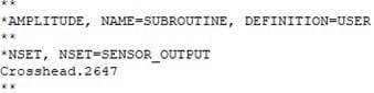
The first thing we need to do is prepare the model to allow a subroutine to interact with it, passing data between the solver and the subroutine. In this case, we’ll use the UAMP subroutine. Some of these modifications can be achieved in Abaqus/CAE, but in this case, we’ll do it by hand. The necessary keyword edits to the basic model are shown below.

To the ‘model data’ of the input file (everything defining the model itself before the step data), we need to define an amplitude, which will be the way the analysis interacts with the UAMP subroutine, and a NSET at the location we want to define a ‘sensor’ to monitor the reaction force. In this case, the control node for the crosshead where the displacement is applied is the obvious location for our sensor.

Now, in the step data for the loading step, we’ll define a dummy CLOAD of zero force for the amplitude to operate on as we’re applying a displacement to the crosshead which follows the default RAMP definition.

And finally, also in the step data for the loading step, we create the sensor history output for the reaction force at the crosshead loading point, in the direction the displacement is applied, which will be passed to the subroutine for the conditional check.

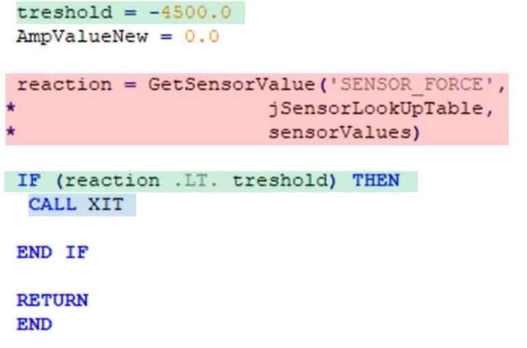
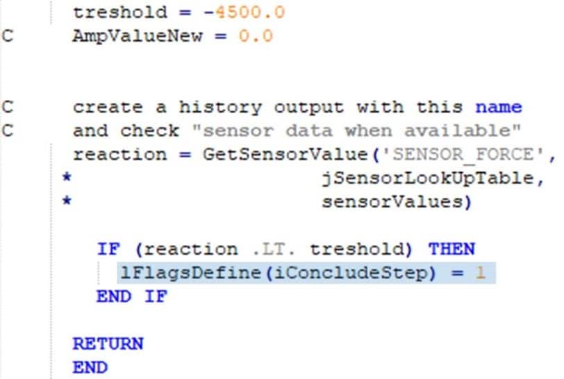
So, now we’ve adjusted the Abaqus input file to pass useful data out to a subroutine. We now need to create a subroutine, using the documented UAMP template as a basis, and add the following statements, which will:

• Extract the sensor data from the solver as each increment of the solution is completed (red box)
• Perform a conditional check on the reaction force to determine if it is less than the target value (green box)
• Loop through an IF statement for each increment of the solution such that once the condition is met, the XIT command is executed, and the simulation terminates (blue box)

The XIT command is recognized by most Abaqus subroutines; we’ve just used UAMP conveniently here to investigate other options later.

Assuming a Fortran compiler is installed and linked to the version of Abaqus executed, we can execute this job with the command line options:

abaqus job=<Job-name> user=<subroutine_name>.f

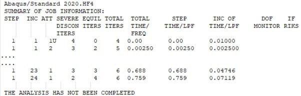
When we run the job, the solution proceeds as normal, until reaching the first converged increment where the reaction force at the sensor node is of a greater magnitude than the user-specified threshold value. At this point the XIT command is executed, and the analysis terminates cleanly.

The status file message “THE ANALYSIS HAS NOT BEEN COMPLETED” is issued as the solver sees that something happened to stop it reaching the end of the loading history.

This is quite neat and easy to set up, but it doesn’t meet our requirements in two ways:

• The analysis terminates at the point where the conditional statement is satisfied. But we really want the step to terminate and the analysis to move on to the unloading step
• The control of the termination point is unrefined, especially with automatic time incrementation applied. At increment 23, the calculated reaction force is -4473 N (just below the termination threshold) and at increment 24, the calculated reaction force is -4598 N (above the termination threshold). So, the XIT command is executed

Approach 2: UAMP Subroutine Utility lFlagsDefine(iConcludeStep)

Improving on the XIT utility, the UAMP subroutine offers a built-in variable that tells the solver to either continue or end a step. By tweaking the subroutine and input file, we can end a step at a specified reaction force and smoothly transition to the next step. This method gets us closer to our goal, but achieving the precise threshold value remains a challenge.

The first thing to observe is that there is a handy inbuilt variable to the UAMP subroutine that we can set, and that the solver knows what to do with.

If we set:

• lFlagsDefine(iConcludeStep) = 0 … the step should continue to the next increment
• lFlagsDefine(iConcludeStep) = 1 … the step should terminate at this increment

So, by simply replacing the XIT command lFlagsDefine(iConcludeStep) = 1 in our subroutine, we achieve the same outcome with functionality already built into the subroutine, not an external command. This is an improvement in functionality compared to XIT, as only the step is terminated, and the solver moves on to any subsequent steps in the loading sequence.

However, in the second/unloading step, the solver simply moves on to the next step as another loading event, as the first step was terminated. So, the jump from a large crosshead displacement at the termination point of the loading step, to zero displacement defined in the unloading step, is too severe to achieve.

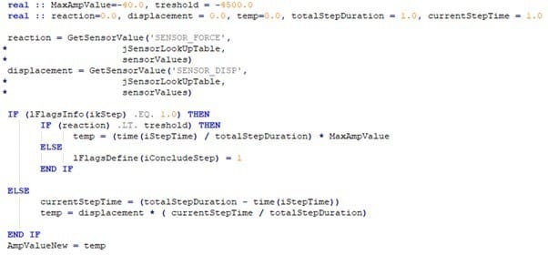
But, with a few tweaks to the input file to control the displacement of the unloading step via an AMPLITUDE that we calculate in the UAMP subroutine, by tracking the step time, total time, and crosshead displacement, we can achieve a process which:

• Proceeds through the loading step to a user-defined threshold value of the reaction force
• Terminates the loading step at the point where the conditional statement is met
• Continues through the unloading step, using the termination point of the first step as the starting point for the second step

When we visualize those results, we do get what we want, but this process could be easier, and more accurate as we still don’t achieve the required termination force exactly.

Approach 3: *STEP CONTROL Keyword

The step control keyword, introduced in the latest Abaqus update, elegantly solves our step termination challenge. With just a couple of lines in the input file, we can define conditions for ending a step and refine the step time as we approach the termination point. This native functionality simplifies our workflow significantly, eliminating the need for Abaqus subroutines and compilers.

To use step control in our workflow, all we need to do to our original Abaqus model of the loading and unloading scenario is:

• Define a reaction force sensor for the crosshead control node natively within Abaqus/CAE or with keywords as we did before the XIT subroutine
• Add the following keywords and options in the history data for the loading step to the input file, as shown below:

These two lines in the input file define the following sequence of events:

• Create a STEP CONTROL definition called STEP_SENSOR to configure some conditional controls to this step (multiple step controls per step are possible)
• In this case, end the step when the conditional statement is achieved, and use automatic step time refinement as the solution gets closer to the termination condition
• The conditional statement that will trigger the end of the step as before: for the reaction force at the crosshead control node we previously defined (SENSOR_FORCE) to exceed a value of -4500 N
• When the sensor force exceeds a value of -4300 N, switch from the automatic step time control defined by STATIC keyword to a more refined fixed time increment so that the step termination point is achieved closer to the required value of -4500 N

Those two lines of a native keyword are taking care of a lot of valuable work. Now, because we don’t need the subroutine, we don’t need a Fortran compiler either, and we can simply execute the job as we would any other, at the command line:

abaqus job=<Job-name>

However, when the loading step is terminated, the solver still moves on to the unloading step. So the jump from the end to the terminated loading step and on to the start of the unloading step is too large for the unloading step to even start to converge.

Thankfully, we can overcome this with more recently added native keywords. This functionality takes the idea of the existing Abaqus restart capability and extends, simplifies, and augments it significantly.

Here’s what we’ll do:

• Create an input file of just the model data and history data for the loading step, including the STEP CONTROL line as shown above, where we terminate the analysis when the same conditional criteria are met (in this case, the keyword option “ACTION = END STEP “ terminates the step, and the whole single-step analysis. But the option “ACTION = END ANALYSIS” is also available)
• Create a separate input file that just contains the history data for the unloading step. (The snippet below is all we need)

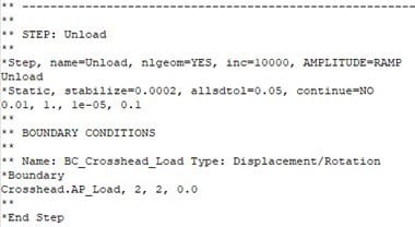
• Create a further input file which just contains the MANIFEST keyword and references the input files for the model data, loading step, and the unloading step

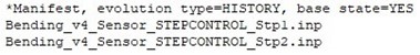
Execute this manifest Abaqus job as we would with any other input file

All the input files referenced under the MANIFEST keyword are then executed in sequence. But, critically, the “BASE STATE = YES” option means that the base state for the unloading step contained in the second input file is the final state of the terminated loading step from the first input file.

Additionally, all the data from the execution of both files is contained within a single Abaqus file structure (the redacted status file is shown below) – including the .odb file.

So, when we interrogate the .odb file for this manifest analysis, everything is available for both steps in one place. This wouldn’t be the case if a restart sequence was created, and additional tools would be needed to combine the odb files.

Do We Still Need Abaqus Subroutines?

The Abaqus solver is continuously improving, bringing advanced capabilities right into the hands of all users through the input file.

Now, adding a touch of autonomy to your Abaqus/Standard analysis is straightforward, even if you’re just getting to grips with the input file basics. And while Abaqus subroutines are valuable tools for many complex tasks, they’re taking a back seat in this particular process.

If you’d like to keep learning about new functionalities in Abaqus, then reach out to the TECHNIA Simulation experts for information about the Continuous Learning Program for Abaqus.