Options to Adapt the Mesh in Abaqus: An Overview

There are different options to adapt the mesh in Abaqus: ALE adaptive meshing, adaptive remeshing and mesh-to-mesh solution mapping. It can be difficult to keep them apart, so in this blog, I’ll give an overview of what they are and what their purpose is. I’ll start with a summary table and then go into more details.

ALE Adaptive Meshing – Repositioning Nodes to Reduce Mesh Distortion

ALE adaptive meshing stands for Abitrary Lagrangian-Eulerian adaptive meshing.

Lagrangian vs Eulerian

With a Lagrangian approach, the mesh moves along with the material. This is what is typically done in Abaqus and for solids in general. With an Eulerian approach, the mesh is fixed and the material moves through it. This approach makes sense for fluids. In Abaqus, a purely Eulerian approach can be simulated using CEL: the coupled Eulerian-Lagrangian method. An example of this can be found in this blog. With ALE adaptive meshing, typically something in between a fully Eulerian and fully Lagrangian analysis is used: the material deforms with respect to the mesh, and the mesh deforms as well: the mesh can thus deform independently of the material.

Purpose

ALE adaptive meshing is usually used to reduce mesh distortion and thus maintain a high-quality mesh even under severe deformations. This is done by moving the nodes. The topology is not altered, so the connectivity and thus the amount of elements is not modified. This limits the remeshing possible.

ALE Adaptive Meshing in Abaqus/Standard

Compared to Abaqus/Explicit, the options for ALE adaptive meshing are a bit more limited in Abaqus/Standard. It can be used

• when no material flows into or out of the domain (Lagrangian approach)
• when material is eroded at the boundary (ablation or wear)

This means that it can be used to reduce mesh distortion on fixed amounts of material. This can improve accuracy and it may even be the only way to obtain a solution in some cases. Furthermore, a boundary mesh motion can be defined independent of the material motion. This is useful in tire analysis for example. The outer surface of the tire is moved inwards, without deforming the material. Part of the material is removed, simulating the wear of the tire.

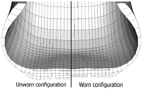
An example of this approach is given in the manual (Tread wear simulation using adaptive meshing in Abaqus/Standard). In this example, wear of a tire is simulated (Figure 1). To prescribe the inwards motion of the boundary of the mesh due to the wear, the user subroutine UMESHMOTION is used.

Figure 1: Worn configuration (obtained using ALE adaptive remeshing) compared to original, unworn configuration. The mesh topology is maintained (node connectivity is unchanged) during mesh smoothing.

ALE Adaptive Meshing in Abaqus/Explicit

With Abaqus/Explicit, Eulerian problems can be simulated as well as Lagrangian problems. This allows a wider range of problems to be analyzed. ALE adaptive meshing cannot only be used to reduce mesh distortion on a fixed body of material, but also cases when material flows into and out of the mesh, that may also deform itself. This is beneficial when simulating processes such as extrusion or rolling. These processes typically lead to large deformations and badly shaped elements. In Abaqus/Explicit, this reduces the time increment and thus increases simulation time besides limiting the accuracy of the solution. Remeshing can improve this.

Compared to Abaqus/Standard, ALE adaptive meshing in Abaqus/Explicit is more extensive. It has several smoothing methods meant for a variety of problem classes, while Abaqus/Standard has a single smoothing algorithm that is intended for smoothing of moved boundary surfaces. It is possible to improve the mesh quality before the deformation begins in Abaqus/Explicit. Also, tracer particles can be defined.

An example of this approach is given in the manual (Forging with sinusoidal dies). In Figure 2 the effect of this technique can be seen: the analysis including ALE adaptive meshing on the right, has better shaped elements than the analysis not including ALE adaptive meshing on the left.

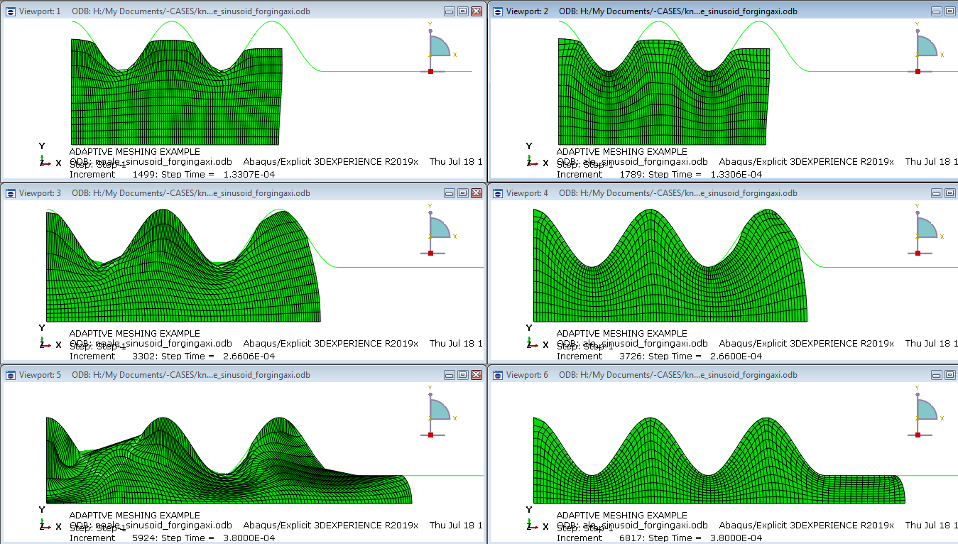
Figure 2: The influence of adaptive meshing in a forging example. On the left results from the model without ALE adaptive meshing are shown, on the right results of the same model but with ALE adaptive meshing.

Miscellaneous

ALE adaptive meshing can be defined on the entire model or on individual parts. Throughout the step, remeshing sweeps are performed; it is thus not necessary to define a new job; the analysis continues with the smoothed mesh. ALE adaptive meshing is available from Abaqus/CAE.

Adaptive Remeshing

When adaptive remeshing is used, the mesh is locally refined in regions where it is needed.

Purpose

While ALE adaptive meshing is primarily meant to reduce mesh distortion, adaptive remeshing is intended to improve accuracy. The same model is run multiple times, each time with a different mesh, while searching for a mesh that fits requirements.

Approach

A model with a nominal – possibly fairly coarse – mesh is defined. Furthermore, a remeshing rule is defined. This remeshing rule fully describes how the mesh should be adapted, including

• the region that is to be remeshed
• the step in which it is to be applied
• error indicators to be used
• the sizing method
• constraints on the remeshing calculations.

Which error indicator(s) are available, depends on the analysis procedure type. For example, there is a heat flux error indicator variable (HFLERI) which is only available when temperature degrees of freedom are present. For mechanical analyses, error indicator variables are defined for element energy density, mises stress, equivalent plastic strain, plastic strain and creep strain. The error indicator is calculated at specified point in time during the analysis, by default the end of the analysis.

The sizing method describes how the element sizes should be changed. Either a uniform error distribution or minimum/maximum control can be chosen. In the first case, Abaqus attempts to meet the target in every element, in the second case only at the location where it is minimal/maximal.

Constraints can be used to limit the element size or number of elements. This can reduce the impact of stress singularities for example.

An example of adaptive remeshing is given in the manual (Thermal-stress analysis of a reactor pressure vessel bolted closure). Results for this analysis are shown in Figure 3.

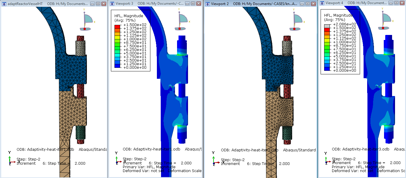
Figure 3: Initial mesh and mesh after 2 remeshing cycles in the thermal model. As can be observed, the mesh is refined in regions where the heat flux is high.

Adaptive remeshing is only available via Abaqus/CAE in Abaqus/Standard. 

Mesh-to-mesh Solution Mapping

With mesh-to-mesh solution mapping, the mesh is replaced by a new one. This can help to overcome mesh distortions.

Purpose

The purpose of mesh-to-mesh solution mapping is similar to that of ALE adaptive meshing: to reduce difficulties due to large mesh distortions. Mesh-to-mesh solution mapping allows a larger freedom of mesh modifications, because it is not limited to meshes having the same topology.

Approach

The analysis is initially set-up as normal. The output must include nodal displacements and restart files must be requested. This allows the solution to be mapped to a new mesh later on. The analysis is run until mesh distortions are so large that remeshing is deemed necessary. A second model is then created, with a new part matching the deformed shape in the original analysis and a new mesh. Abaqus does not create such a mesh or part for you. (Extensive) manual effort is required to obtain this. Once the original analysis and the new mesh are available, the solution from the old analysis can be mapped to the new mesh. This is only possible using keywords.

The rest of the model must be defined as well. Loads and boundary conditions are not automatically carried over to the new mesh: it is a new analysis in which the initial state of the model is obtained from a different analysis. For consistency, at the start of the analysis with the new mesh, the loads and boundary conditions should match those in the previous analysis.

In Figure 4 results are shown for a simple uniaxial compression case. When the uniaxial compression is large, the elements become distorted: the width is much larger than the height. Mesh-to-mesh solution mapping is used to transfer the results to a new mesh, with square elements. As can be seen in the images, the stress nicely matches the mapped stress, while the strain is taken with respect to the new state of the model.

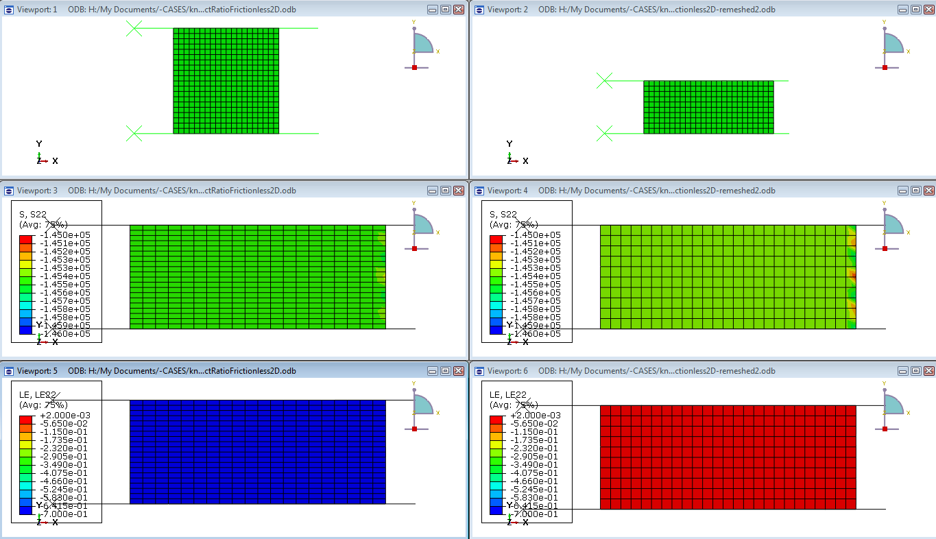
Figure 4: An example of mesh-to-mesh solution mapping. The left images show the original mesh, the right images the new mesh. The initial shape is given on the top, the stress (vertical component) is shown in the middle images and the strain (vertical component) on the bottom images. The same scales are used for the original and the new mesh.

When the material is further compressed in both cases, the stress lines overlap (Figure 5).

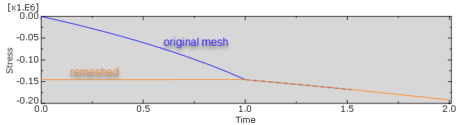
Figure 5: Stress in an element in the original mesh and in the remeshed case. During the first second in the remeshed analysis, an equilibrium solution is obtained. After this point in time, the analysis continues using the same boundary conditions as the original.

The strain lines have an offset (Figure 6).

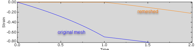
Figure 6: Strain in an element in the original mesh and the remeshed case. During the first second in the remeshed analysis, an equilibrium solution is obtained. After this point in time, the analysis continues using the same boundary conditions as the original. Strains are calculated with respect to the initial state of the new mesh (which does not match the original mesh).

Mesh-to-mesh solution mapping is only available in Abaqus/Standard.

Conclusion

Within Abaqus, different techniques are available to adapt the mesh. Which one to use depends on the intended application. When the intent is to obtain a converged mesh, then adaptive remeshing is most appropriate. This is only available in Abaqus/Standard. When the intent is to reduce mesh distortion, then for Abaqus/Explicit ALE adaptive meshing is the way to go. ALE adaptive meshing is also suitable in Abaqus/Standard for analyses where material is removed from the outside such as wear. For larger mesh changes intended to reduce mesh distortion in Abaqus/Standard, mesh-to-mesh solution mapping can be investigated.