Offshore and subsea structures have been constructed and commissioned for many decades now, resulting in quite innovative and mature technologies.

These structure types are subjected to loads of different nature. Therefore there is the need for developing methods, that allow for a structural assessment under serviceability loads, in a quick but also accurate way.

Particularly, for subsea structures focused on oil extraction from reservoirs, lying under the seabed, interaction with the surrounding soil becomes of critical importance.

In this blog post, we will be investigating a drilling wellhead under external load action while also incorporating the behavior of the surrounding fully saturated soil from the seabed, in terms of nonlinear springs.

The wellhead is a drilling component typically used in the oil and gas industry (Figure 1).

Figure 1: Wellhead representation 

This component is subjected to hydrodynamic loads and also structural loads from the seabed acting normal to the symmetry axis of the wellhead. Those seabed loads generated due to the Soil Structure Interaction (SSI) are relatively high and of cyclic nature. Since the wellheads, typically incorporate welds, it becomes of crucial importance, establishing a method, to adequately predict stress levels at various locations along the height of the wellhead (locations where welds are present), so that the respectful welds can be assessed for fatigue.

If this is not done in an accurate manner, the component can fail and even salvaging it can be proven to be impossible (and surely costly) due to its operating environment.

In terms of modelling Soil Structure Interaction (SSI) in the finite element analysis world, various modelling approaches can be deployed. To my knowledge, in terms of available methods, two are the most popular:

Method 1: Modelling the surrounding soil’s behavior with non-linear springs ( simplified, computationally cheaper).

Method 2: Modelling the surrounding soil’s behavior  by including the soil geometry and modelling it as a continuum (more complex, computationally more expensive).

For this blog post, we will be investigating method 1. Method 2 will be covers in another future blog.

Model Geometry

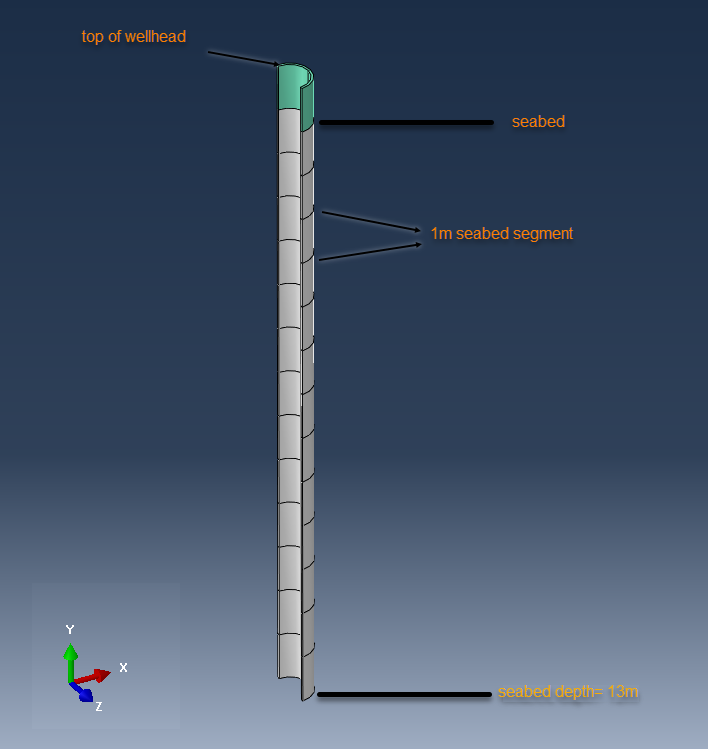
The geometry that was used for this example is shown below, in Figure 2. Half symmetry was used in the analysis.

Figure 2: Model Geometry

The top 1m segment represents the top of the wellhead (green color), rising 1m over the seabed. Under the seabed, the segment of the wellhead (white color) that has been modelled is 13m. The wellhead’s outer diameter is constant=1200 mm and its thickness t= 60 mm.

Material

Wellhead component

In terms of material modelling, the wellhead’s material is steel, and the material law is linear elastic, with an E-modulus equal to E=210GPa, and a Poisson’s ratio equal to ν=0.3.

Soil

As for this blog post, we will not be modeling the soil as a continuum (explicitely), but rather with the use of nonlinear springs, we need an analytical equation that can adequately describe the Soil Structure Interaction (SSI), in terms of the lateral soil resistance vs lateral soil deflection (load vs displacement).

A widely used analytical relationship that allows for this, is the P-y relationship.  Typically, this relationship is empirical, and it takes various forms based on the type of soil (soft clay, stiff clay etc.).

This relationship essentially calculates the ultimate resistance of the soil (Pu)and relates it with the actual lateral soil resistance P.

The P-y relationship depends on the following:

• the type of soil being investigated
• the material parameters of the soil (derived via testing)
• the depth under the level of reference (seabed level in our example)

For our example, a single soil layer of soft clay was used, but of course multi-layered soils can be implemented, provided that the respectful P-y curves correspond to that specific soil type and material parameters.

Figure 3, shows the equations used for generating the P-y curves (and consequently inputting them in Abaqus).

Figure 3: Equations used for P-y curve generation (soft clay)

The equations shown in Figure 3 correspond to soft clay. The complementary material parameters used are exemplary. Typically, those parameters are extracted from the literature or derived by soil testing. Others, such as J, are empirical (typically 0.25<J<0.5).

Figure 4 shows a sketch of the lateral resistance effect on a pile under lateral loading (top view).

Figure 4:sketch demonstrating soil’s resistance under lateral loading (P-y method)

Figure 5 shows the nonlinear P-y curves of our example, for soft clay, for various depths under the seabed.

Figure 5: P (N/m) -y (m) curves for soft clay at various depths

Nonlinear spring modeling in Abaqus

In Abaqus linear springs are typically modelled either with spring elements ((Assembly-based modules-->Special-->Spring/Dashpot) or with the use of a linear connector with elasticity (spring constant) applied to it.

Since the P-y curves have a nonlinear form, connector elements will be used, in order to capture this behavior.

Spring discretization

Figure 6 shows details from the process of setting up the nonlinear springs. In specific, 13 springs will be created, all of them representing the soft clay’s lateral resistance. The only parameter changing per spring (for the P-y curve input) is the depth under the seabed.

Figure 6: Nonlinear Springs locations

The uppermost plane in figure 6 represents the seabed level (y=0). The wellhead ontop is hidden to enhance visibility.

We first need to create 13 Reference Points (RPs) that lie, at the symmetry plane (x=0) and at a proper location. The wellhead geometry needs to be partitioned (in 1m segments) as shown in figure 6. Then the RP per segment,needs to be located halfway through (at 0.5m of a 1 m segment, so RP20 =0.5m, RP22=2.5m). This RP coordinate is  the depth that will be used in the Pu equation (first equation -figure 3).

Next, in order to be able to assign our connector behavior, we need to create wire features for all 13 RPs. Those wires will be connected to ground, as shown in Figure 7.

Figure 7:Wire features for RPs connected to ground

Figure 8 shows a detail from the connector section creation as well as the connector type that will be used to model the non-linear load-displacement relationship.

Figure 8: Connector Section creation

Figure 9 shows the continuation of the connector section creation from Figure 8. Specifically, a Cartesian Nonlinear connector needs to be created and the respectful P-y curve needs to be given as input.

Figure 9:Connector Section creation cont.d

The detail in Figure 9, shows the load-displacement input corresponding to the spring in my analysis, situated at 4.5 m (RP location) under the seabed. Bear in mind that the units in the P-y equations of Figure 3, are N/m for P, and m for y.

In Abaqus however, a Force (N) vs lateral displacement y(m) needs to be given as input. Therefore you need to multiply the P-y curve with the total spring range. As in our analysis, each spring expands in sections of 1m, we can input the data pair directly without worrying about having to rescale the curve (since our spring range is always equal to 1). 

Since we are modelling a single soil type only (soft clay) in this example, you can also use fewer or more springs if necessary, as long as you remember to multiply the P-y data input with the geometry segment (range) to which the spring corresponds. This needs to be done also in a case where you are modelling a multilayered seabed/soil, with each soil type present over different depth ranges.

We need to input all 13 P-y curves by creating 13 connector sections that will be assigned next, to the 13 wire features. A detail of this process is shown in figure 10.

Figure 10:Connector Section assignment on wire feature

Now that our nonlinear connectors are representative of the soil type and depth characteristics, we need to couple the nonlinear connector springs that are grounded, to the surrounding wellhead geometry. As mentioned, 13 springs will be used in total, each one coupled to the surrounding wellhead, spanning across a depth of 1m (per spring).

Figure 11, shows a detail of the non linear connector coupling to the surrounding wellhead surfaces. It is noted that the exterior wellhead surfaces need to be coupled to the nonlinear connectors. This coupling is implemented via distributed couplings.

Figure 11:spring-geometry coupling detail

Mesh

A mesh detail of the discretized geometry is given in Figure 12. No mesh convergence study was performed, and C3D8I elements were used.

Figure 12: Mesh detail

Loads & BCs

In terms of external loading, there is a concentrated force acting on top of the wellhead (+X direction) as well as a moment (-Mz). Both loads are applied on a single RP, located at the symmetry plane, that is coupled (via a distributed coupling) to the uppermost surface of the wellhead. This is shown in Figure 13.

Figure 13: Load types and coupling

In terms of boundary conditions, we have the symmetry conditions (Xsymmetry) and we also constrain the lowermost edge (semi-cycle) of the wellhead in the Y direction. This is shown in Figure 14.

Figure 14: Boundary Conditions

Results

The results will be evaluated in terms of Von Mises Stresses (in MPa) and lateral displacements (U1 in mm) against the distance from the top of the wellhead (where the remote loads are acting).

Those results will be extracted from the location shown below, in Figure 15.

Figure 15: Path for output and von Mises stress detail

Von Mises stresses and lateral displacements are shown below, in Figure 16. It can be seen that for the type of soil and external loads applied, the von Mises stresses become equal to zero, at approximately 8 m below the seabed level.

Figure 16: Von Mises (MPa) and lateral displacement U1 (mm) results

So, if for example there is the need to assess a weld in terms of fatigue against a code, the engineers can read the von Mises stress values at the corresponding depth where the particular weld is present.