Tank Droptest – First Steps on the 3DEXPERIENC Platform

In this blog we’ll do an FSI droptest – on the 3DEXPERIENCE Platform. We’ve done something similar before in Abaqus. Doing it on the platform will give an idea of its user interface and capabilities.

The Result

Let’s start with the end result, so you have an idea of where we’re going:

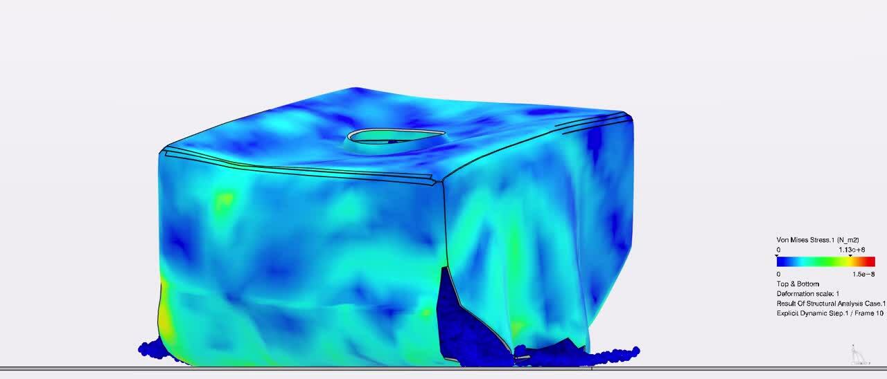
Looks pretty cool, right? This is a water-filled HDPE tank that is dropped from a height of 40 m.

The tank is modelled using shell-elements. The HDPE is modelled as a elastic-plastic material with damage. The water is modelled using SPH. For the material definition, an equation of state is used. The floor upon which it is dropped is considered rigid. The falling part of the drop is not simulated; instead, an initial velocity is specified. Gravity and contact are included.

Let’s take a look at how this is set-up on the platform now.

The Process on the Platform

On the platform, performing an analysis is divided in three aspects. Each aspect has one or more apps related to it. The three aspects are model, scenario and results. We’ll go through each of these.

Prerequisite – Geometry Import

First the geometry is imported, in this case from a SolidWorks assembly (tank and floor) and a step file (water). Using the CATIA Assembly Design app, the water is added to the rest of the assembly.

Model

While selecting the product at the top of the tree, the Structural Model Creation app is opened to define the model set-up. We can select the shapes that will contribute to the model (in this case all of them). An impression of the user interface is shown in Figure 1.

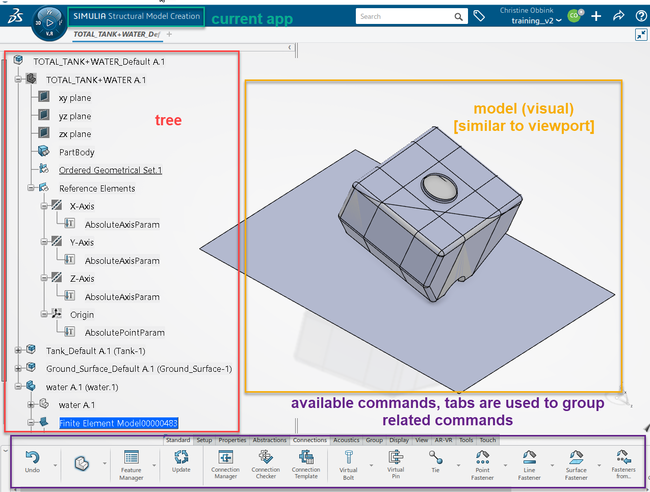
Figure 1: the 3D Experience user interface, indicating the location of different features.

Material and Section Definitions

Both materials and sections need to be defined. In contrast to Abaqus, it is not necessary to first create a material, then a section referencing that material and finally assigning the section to a piece of geometry: materials can be assigned directly to the geometry. The section definition will then refer to applied material.

Materials

The concept of defining materials is very similar to Abaqus, though the user interface looks different (Figure 2)

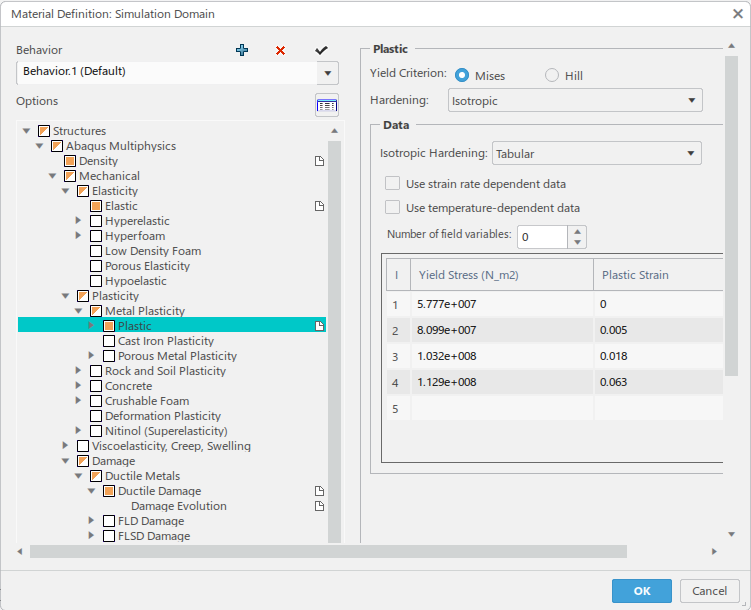
Figure 2: Defining material properties.

A few remarks:

• The platform uses units. You can therefore specify the (material) input data using a unit of choice. When you include the unit, it will automatically be converted to the default units for the current model. What these defaults are can be selected by the user.
• It is possible to define multiple behaviors for a single material. This could for example include a linear elastic and an elastic-plastic behavior for the material. You can select which one to use on a case-by-case basis.
• Since this is part of the platform, all material definitions are stored in a database. You can search this and easily reuse data defined earlier. Of course, this may lead to multiple materials that all have the same name. The search functionality allows you to easily see the properties of each material, to make a sensible choice.

Sections

Sections are created from the properties tab (Figure 3). We’ll use the shell section (tank, floor) and SPH Particles (water) sections here.

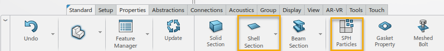
Figure 3: Options for defining sections.

In the section definition we need to define a support. Different methods are available, including face propagation. This is used to select all faces within a certain angle of each other to easily select the entire outer surface of the tank (Figure 4).

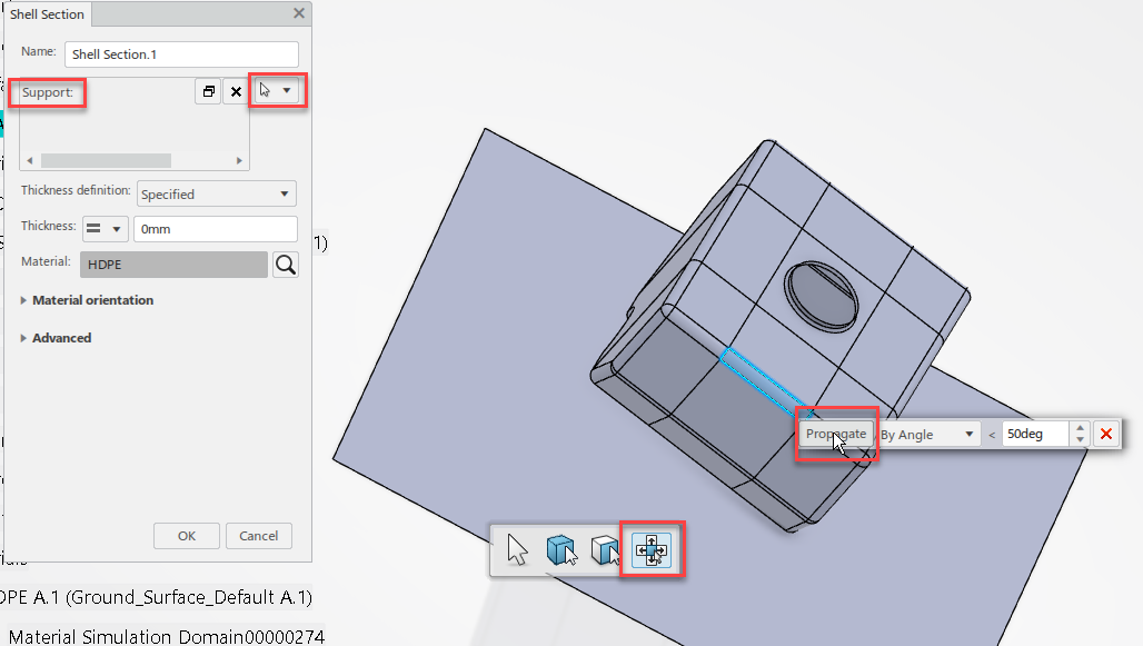
Figure 4: Using the face propagation tool to select the support for the shell section.

All faces included as support are listed and can be individually selected and removed if necessary. As usual, the shell thickness is defined. Offsets and material orientations can be defined if needed.

Different aspects of the model can be shown/hid by right-clicking them in the tree and selecting show/hide. This can be used to show the water part and hide the rest.

The SPH Particles tool is used with the water part as support, to convert the mesh in this region to SPH Particles. In this case the background grid option is used, and the grid size is specified (Figure 5).

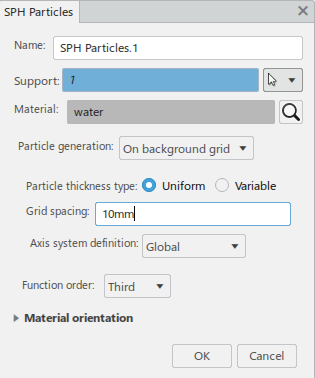
Figure 5: SPH Particles definition

This is more intuitive than doing the same thing in Abaqus. In Abaqus, converting elements to particles is specified from the element type definition. The background grid option is not available from the CAE and needs to be added via keywords in the section controls.

Rigid Body Definition

The floor is modelled as a rigid body. This is selected from the Abstractions tab in the Structural Model Creation app. This means the rigid body is part of the model definition, not of the scenario. The floor is selected as support. It is not necessary to manually specify a reference point; it is also possible to use the center of mass (Figure 6).

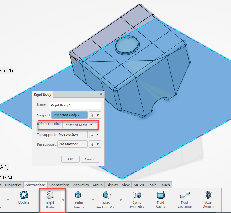
Figure 6: Defining a rigid body

Mesh

Geometry can be meshed on assembly level or on part level. A combination can be used in a model. Multiple meshes can exist for the same geometry, in this case the user needs to select the FEMrep (FEM representation) to be used.

The way a mesh is defined is quite different compared to Abaqus. For this post, it does not make sense to go through all the options. In general, there are options available during meshing on the platform, that would require geometrical changes in Abaqus. Some examples:

• Meshing over holes/small geometry
• Capturing existing meshes: from the mesh module you can decide whether geometry at the same location/close to each other should share nodes or not
• Selecting a minimum angle between faces to determine whether edges are included in the mesh or not (similar to virtual topology)

In this example, the second point is most relevant: capturing existing meshes.

If we do not select this option, then the different faces do not share nodes (Figure 7).

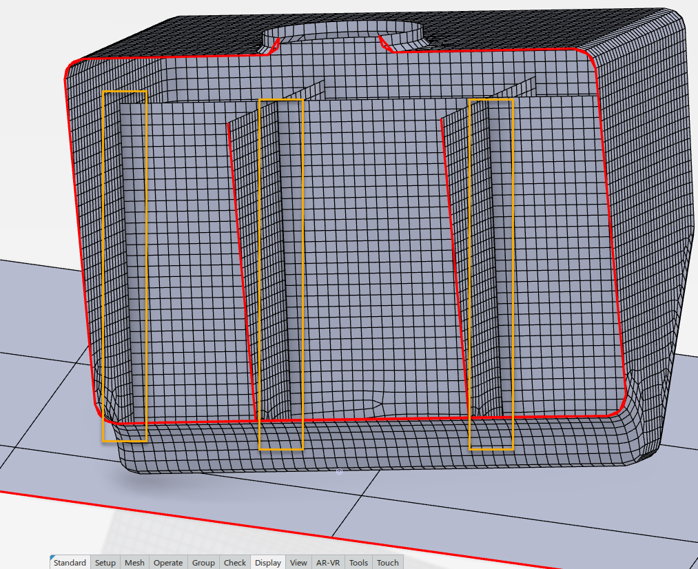
Figure 7: Example of mesh where mesh capture is not selected.

By changing the mesh options (without changing the geometry) the mesh can be made so that nodes are shared (Figure 8).

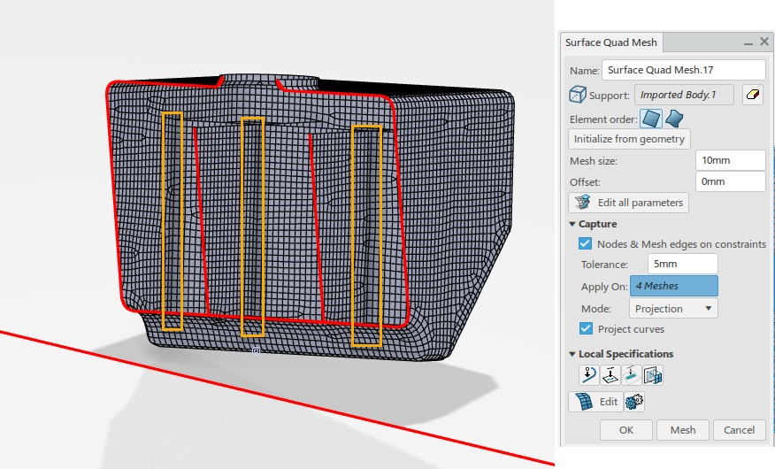
Figure 8: Example of mesh where existing meshes are captured. The mesh on different faces that are near each other now share nodes.

This can be fully controlled, selecting where the mesh should or should not be captured. When meshing is done on assembly level, the mesh of a nearby (but different) part can also be captured.

Scenario

The scenario is defined using the Mechanical Scenario Creation app. This is the most extensive scenario app. It includes Abaqus/Explicit, which will be used here. The scenario is defined within an analysis case. It is possible to define multiple analysis cases and to create a new analysis case by duplicating an existing case.

The things that can be simulated are similar to what is possible in Abaqus (which makes sense because the same ‘engine’ is used to solve things), but the way different options are accessed differs a bit. There are tabs to access different types of options such as procedures, initial conditions, interactions, restraints, and loads. Here ‘restraints’ refers to fixed boundary conditions and ‘loads’ to things that cause deformations: both applied displacements and different types of forces.

As can be seen in Figure 9 the options tend to be more specific than in Abaqus: there is for example a ‘clamp’ option, which restricts all degrees of freedom and a ‘planar symmetry’ option that applies symmetry conditions. It is not necessary to specify the symmetry plane for faces; this is automatically detected.

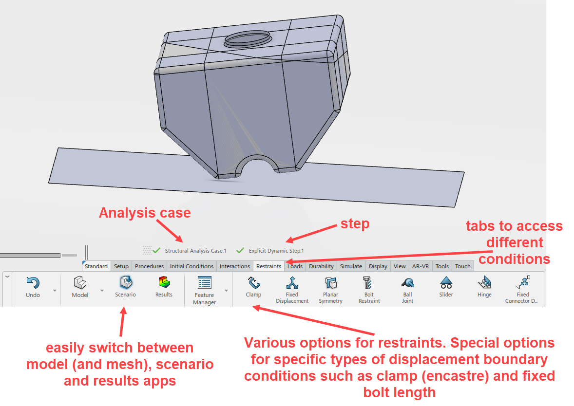
Figure 9: Example of Mechanical Scenario Creation app interface.

In this case, an initial velocity is applied to the water and the tank, gravity is applied to the entire model, general contact is defined, and the rigid body is clamped (Figure 10).

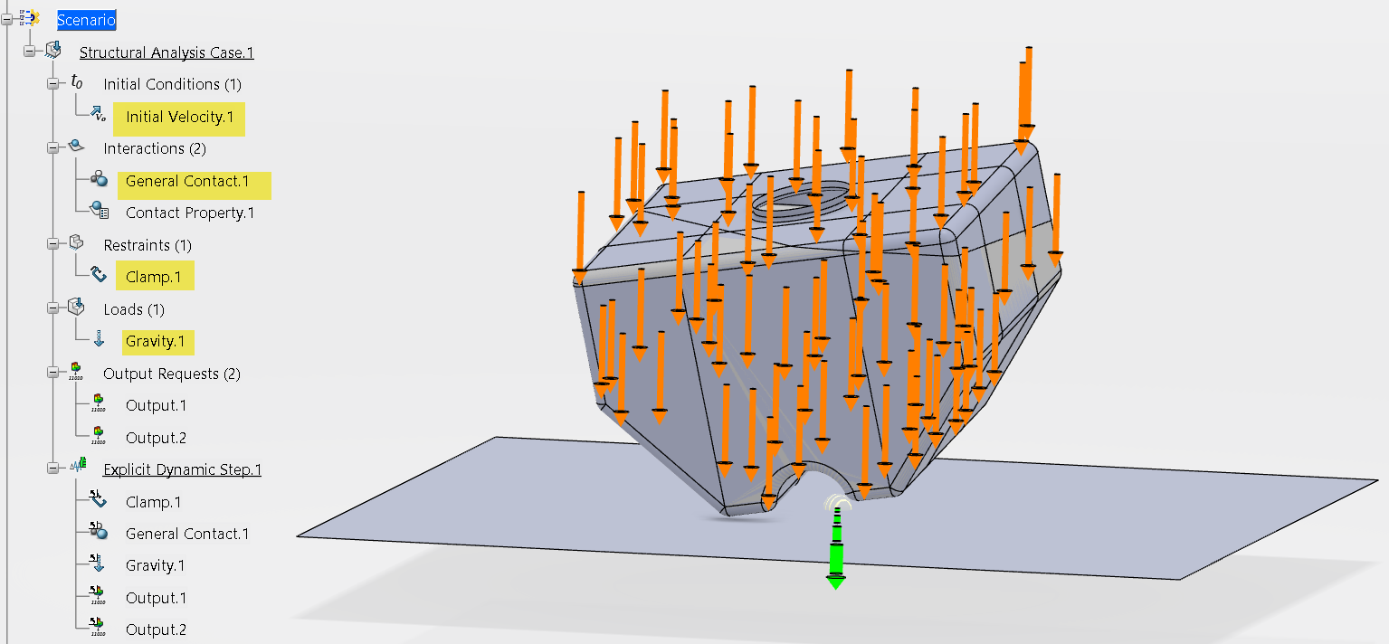
Figure 10: The applied scenario

The clamp can be applied directly to the rigid body, without needing to define e.g. a set there, but selecting from the FEM Feature Selection (Figure 11).

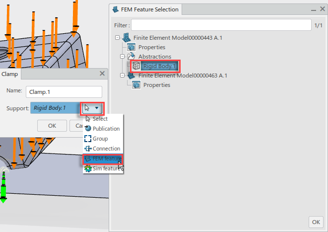
Figure 11: Defining the support for the clamp by selecting the rigid body from the FEM Feature Selection.

The Run

The analysis can be run by selecting Simulate from the Simulate tab (Figure 12).

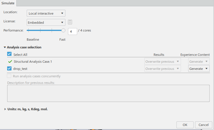
Figure 12: The simulate dialog box.

Here you can choose which analysis case to run, whether to overwrite previous results and what units are to be used in the analysis. These units may differ from the ones used while setting up the analysis. They should be consistent.

By the way: this is only possible if something has changed to the analysis, otherwise the system will notify you that the results for all analysis cases are up to date and it will not run the analysis again. A nice feature, but not very handy if you want to show the user interface in a blog 😉

When the analysis is running, you can monitor the progress and check the .sta, .msg files etc. Once it is finished, the Physics Results Explorer App is opened automatically. Results can be viewed here.

Results

There is a lot that can be said about the possibilities in this app. I won’t even try to be complete, but just mention a few things that got my attention, since they differ from Abaqus. To my knowledge most/all of the visualization options in Abaqus are available on the platform as well.

• Plots are stored. By default a number of plots is created, including the undeformed and deformed model, displacements and von Mises Stress. Settings such as the quantity plotted, the display group, whether displacements are shown and whether shell thickness is shown are stored as part of the contour plot. These are available from the tree, so you can easily switch between different plots. This does not include model view and active frame by the way.
  
  
• Legends indicate the minimum and maximum values in a contour plot and can be both horizontal and vertical (Figure 13).
  
  
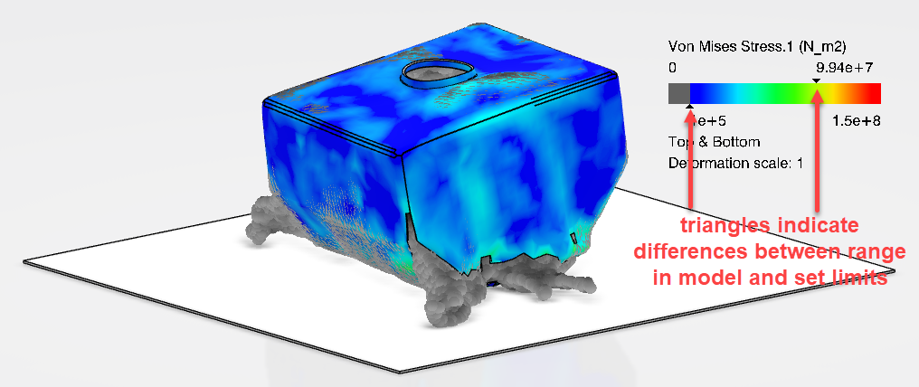
  Figure 13: Contour plot with horizontal legend. The difference between the user-defined legend range and the range in the model is indicated with triangles. The legend can be moved around and resized, similar to the model itself.
  
  

• Sensors allow you to easily determine maximum/minimum/average/etc. over both space and time.
  
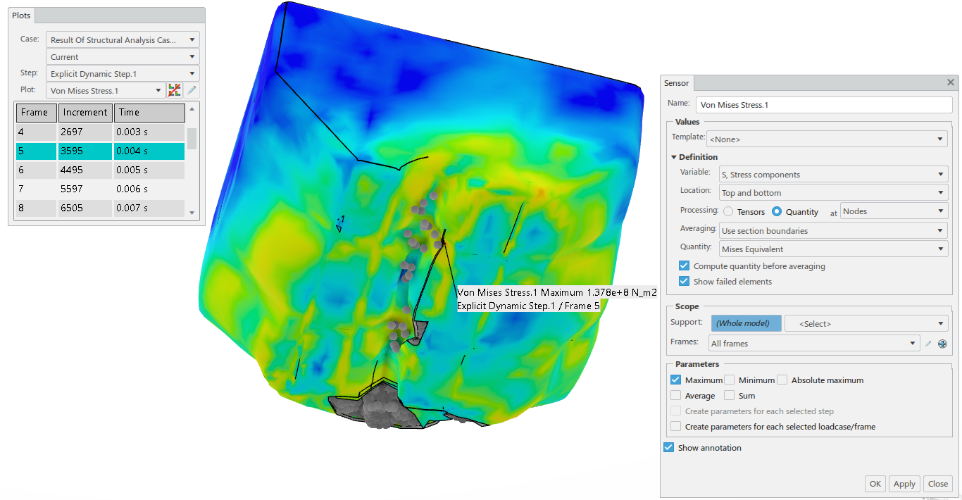
  Figure 14: Example of a sensor, in this case showing the maximal von Mises stress. The frame where the maximum occurs (frame 5) is selected.
  
  

• It is possible to visualize more than one maximum (Figure 15). The annotations can easily be moved around.
  
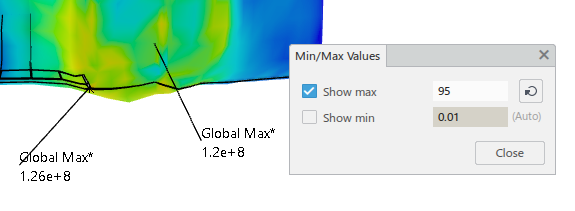
  Figure 15: Segment of the tank with two global maxima (top 5% of stress) shown.
  
  

• There is an option to create automatic reports. You can select the information to be included from a drop down list such a different views, the model set-up, amounts of elements, plots, results from sensors, etc.

Conclusion

So, what is my impression comparing simulation on the 3D Experience platform to Abaqus?

• The geometry set-up and meshing require some adjusting. At first glance, there seem to be nice and useful options to make meshing more controllable, reproducible, and efficient. It will take time and effort to learn to fully use them though. This might be a nice topic for a future blog.
• Having Abaqus-knowledge, the scenario set-up is fairly straight-forward. Most Abaqus functionality is included. Where to find which function is quite intuitive. Some options are easier to find and define on the platform compared to Abaqus because the tools are separated more and labelled more specifically.
• The results look nice and clean. The most common plots are easily and intuitively created. Learning to make the most out of the options will take additional time, but I expect it would be worth it.
• Switching between different apps is straight-forward, once you get the hang of it.
• As can be expected there are extensive options to ensure geometry is not modified unnecessarily to perform simulations and to keeping track of different versions.