While Abaqus is used most for mechanical analysis, there are other options as well. Thermal analysis is one of the possibilities. In this blog, I will show how to set up such a thermal analysis using Abaqus.
Example
As an example I’ll use something I’ve been wondering about for some time, related to baking home-made brownies. I’ve baked brownies in a metal pan numerous times, and this works out well. However, when switching to a different oven that did not fit the metal pan, I used a silicone version instead. (It was more flexible so it did fit inside the oven.) Unfortunately, this did not work out well: even after increasing the baking time, the batter remained raw at the bottom of the pan more than once. I’ve always suspected that the silicone pan was causing the issues, the material properties of steel and silicone are pretty different after all. Luckily I have a larger oven now, that does fit a metal pan, and last time I tried with a metal pan, the brownies turned out as they should. To improve understanding of what is going on, I will set up a simple simulation.
Geometry
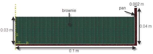
As with a mechanical analysis, we need to define the geometry. Though my actual brownie pan is rectangular, I don’t expect results to be much different in a circular pan, while running times will be much less when using an axisymmetric assumption. So, keeping in mind that a model should be as simple as possible (but not simpler) the axisymmetric geometry shown in Figure 1 is used. The pan and the brownie are separate parts. Regular SI units (m, kg, etc.) are used for the model.

Figure 1: The meshed geometry used for this thermal analysis.
Mesh: Element Type
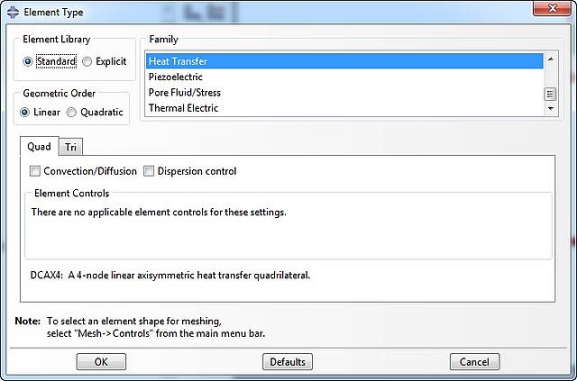
Meshing is also similar to meshing for a mechanical analysis, so the parts are first seeded and then meshed. The main difference is the element type used: we will use elements of the heat transfer family (Figure 2). These have a single temperature degree of freedom, instead of displacement degrees of freedom.

Figure 2: Element type selection.
Material Properties
The equation that governs this purely thermal analysis is:

Here ρ is the density, c is the specific heat, T is the temperature, t is time, k is the conductivity and x is place. Therefore the density, specific heat and conductivity of the materials are required, while a mechanical stiffness is not. For steel and silicone, more or less reasonable properties could be found on the web. As I expected, the thermal properties of brownie batter aren’t as readily available. There is actually more data on simulating baking of bread, cupcakes etc. than I expected, and I decided to use values for cupcakes/yellow cake. Of course this won’t be completely accurate, but it is probably sufficient, keeping in mind that currently our main purpose is to get a better understanding of what is going on; not to calculate exact values.
The following properties are used:
|
|
Steel [1]
|
Silicone [2]
|
Brownie [3]
|
|
Density [kg/m3]
|
7832
|
1700
|
500
|
|
Specific heat [J/(m s ̊C)]
|
434
|
1175
|
2550
|
|
Conductivity [J/(kg ̊C)]
|
59
|
1.375
|
0.15
|
The brownie properties as assigned to the brownie. The analysis is performed twice: once with steel properties assigned to the pan and once with silicone properties assigned to the pan. This is the only difference between both analyses.
Step
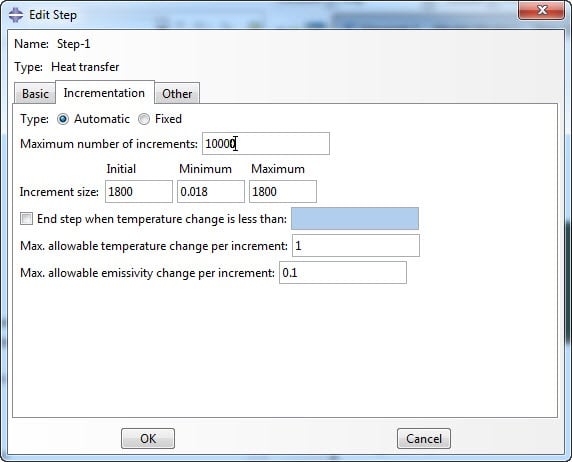
A step of type ‘heat transfer’ is used. The transient response is taken into account, to see how the brownie heats up in the oven as opposed to the steady state that may be reached when the brownie would be in the oven for an infinite amount of time. The time period is 30 minutes or 1800 seconds, about the time the brownies need to be in the oven to bake them. Automatic time increment is used and the maximum number of increments is increased from the default 100 to 10000. The maximal allowable temperature change per increment is set to 1 ̊C (Figure 3).

Figure 3: Editing the heat transfer step.
The time increment will then automatically be chosen in such a way that the maximal change in temperature in an increment does not exceed 1 ̊C in any node (unless boundary conditions prescribe this). This thus influences the accuracy of the analysis in time.
Contact
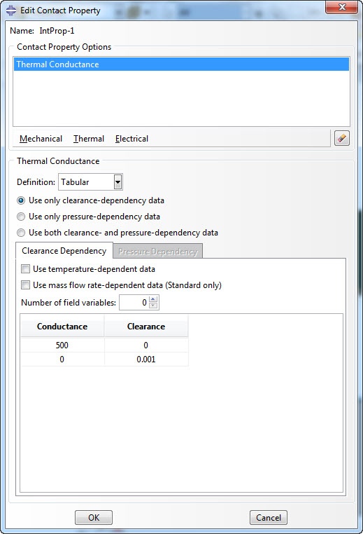
The brownie and pan are separate parts and heat transfer bewteen them should be possible. To allow this, an interaction is defined, in this case surface-to-surface contact. This requires interaction properties: thermal conductance is defined. Conductance depends linearly on clearance. A conductance at 0 clearance as well as a clearance at 0 conductance are specified (Figure 4).

Figure 4: Defining thermal conductance.
Assigning this interaction property to the interaction, allows heat transfer between the brownie and the pan.
Influence of Oven
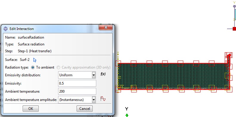
During baking, the brownie and pan will heat up in the oven, mainly due to radiation. A thermal flow needs to be applied to simulate this effect. In this case, we will use an interaction of type Surface radiation. With this option, a heat flux is applied to a surface according to the formula:

Here q is the heat flux across the surface, ε is the emissivity of the surface, σ is the Stefan-Boltzmann constant, T is the temperature at this point on the surface, T0 the ambient temperature and TZ is the value of absolute zero on the temperature scale being used. Though this is meant to simulate heat loss due to radiation, we will use it here to model heating up due to radiation, because it is a simple way to provide a more or less reasonable heat flux.
The ambient temperature is assumed to be 200 ̊C, the temperature inside the oven and the radiation is applied to all outer surfaces (Figure 5).

Figure 5: Defining Surface radiation.
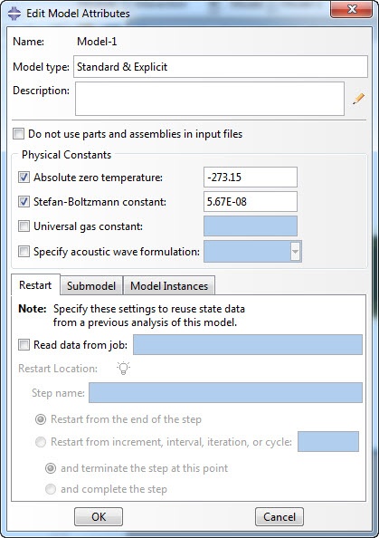
Because you do not specify the units used in Abaqus, but have to work with consistent units, Abaqus does not automatically know what the value of the Stefan-Boltzmann constant or the absolute zero temperature should be. There need to be defined as model attributes. By right-clicking the model in the model tree the ‘Edit Model Attributes’ dialog box pops up. Here these values can be specified (Figure 6).

Figure 6: Specifying the Stefan-Boltzmann constant and absolute zero temperature as model attributes.
Results
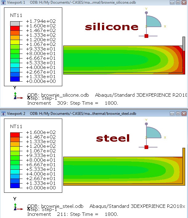
As the default output requests are deemed sufficient, we can now create and run the jobs. As can be seen in the movie and in Figure 7, the results for steel and silicone are actually not that different. The temperature gradient with the silicone seems a bit larger, but the difference in thermal material properties by itself does not seem to explain why baking brownies in a silicone pan would fail.

Figure 7: temperature distribution after 30 minutes.
Video showing animated temperature distribution results.
So now what? Is the model too simple? Do we need to include other differences between silicone and steel, such as a difference in the heat flux towards the material or the thermal contact properties? A quick internet search does not result in other people complaining about brownies failing in silicone pans, which I would expect if it is a general issue. Also, I’d never performed a nicely controlled experiment, using the same recipe and oven with a silicone and a steel pan. Perhaps other differences than the baking pan were causing the problems. While simulations can give a lot of insight, experiments are necessary as well. So, in this case I decided to bake brownies in the silicone pan using an oven and recipe that I know produces good brownies with a steel pan.
And guess what?
They turned out fine.
Conclusion
So, in conclusion, I’ve given an example of how to set up a thermal analysis in Abaqus. And apart from that, I myself have learned that while the thermal properties are actually quite different, both steel and silicone can be used for baking pans. My assumption that silicone baking pans are not suitable to bake brownies is therefore BUSTED.
[1] https://www.engineersedge.com/properties_of_metals.htm [steel SAE 1010]
[2] https://www.azom.com/properties.aspx?ArticleID=920
[3] http://article.sciencepublishinggroup.com/pdf/10.11648.j.abb.20140202.12.pdf


