Use Mesh-independent Fasteners to Simulate Connection Points in Abaqus

In Short:

• Mesh-independent fasteners couple layers of material to each other, simulating the effect of e.g. spot welds.
• They don’t require the coupled region to be separated from other regions by a partition (mesh-independence), making them easy to define.
• Instead their position is defined by attachment points, reference points or nodes.
• It is possible to create patterns of attachments points, to easily define the location of multiple fasteners.
• Fastener are defined from the interaction module, via “special”, “fasteners”, “create” or the “create fasteners” icon.
• Rigid MPC fasteners are possible. The behavior of the fastener can also be defined via a connector section to allow more complex behavior.

Introduction: Approaches to Simulate Point Connections

Often two (or more) parts are connected at specific points, for example by a number of screws along a line. In a simulation, the connection needs to be taken into account.

Depending on the level of detail required, different approaches are thinkable. On a coarse scale, the parts can be tied to each other throughout their contact surfaces. This is simple to do, but it does not match reality very closely.

If we do want to take into account the discrete locations of the connection points, we can partition the surfaces that are connected by the screws at the position of the screws, define surfaces there and tie these to each other.

It would probably also be possible to simulate the screw itself, but unless the screw is the main topic of investigation and only a limited number of screws are simulated, this is not feasible.

An alternative approach is to use fasteners. One of the advantages of this approach is, that it is not necessary to specify the connection region as a surface. Instead, it can be defined as a point (an attachment point, reference point or node), with a given radius of influence. This makes meshing a lot simpler and faster.

In order to make a better choice between the fastener approach and the tie approach, we compared the approaches in a simple example problem.

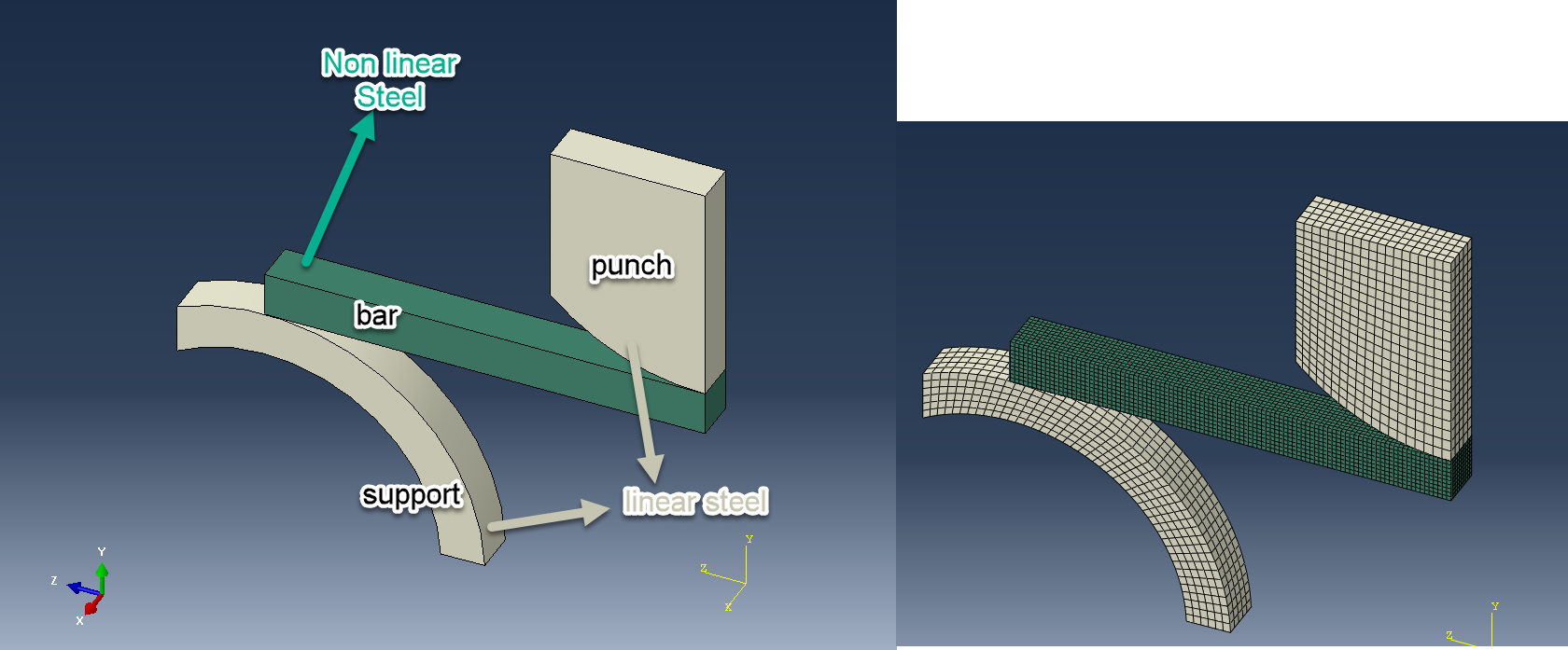
Example Problem: Bending of a Panel Screwed on Top of a Frame

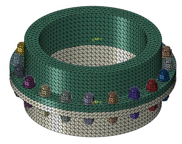
As an example problem, we took a section of a panel screwed to a frame on both sides (Figure 1). Two screw positions are included on each side. This was deemed the minimal amount to simulate a line of screws. In this example, the sides of the frame not connected to the panel are completely fixed (no displacement in any direction) and the opposite end of the panel is loaded with a vertical force via a reference point and coupling.

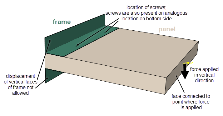Figure 1: Set-up of the example model.

Approach 1: Tie of Partitioned Faces

As a first approach, the parts are connected by tying surfaces corresponding to the screw locations to each other.

This requires partitioning the geometry so that these surfaces can be defined. The faces of both parts are partitioned, so a circular region corresponding to the screw is defined. These regions are small compared to other dimensions even in this example (Figure 2).

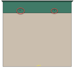
Figure 2: Top view of the assembly show the size of the screw locations.

For an actual analysis, the parts analyzed would be much bigger, and there would be much more screw locations. Partitioning a region for each screw would require quit a lot of manual labor then. Furthermore, the mesh needs to be refined enough to describe this small circle. Because of this, very small elements are needed, at least locally around the screw region. The meshed used for this example, is shown in Figure 3.

The corresponding surfaces on panel and frame have to be tied to each other. This can be done by making a surface corresponding to all screw locations on the frame, and a second surface corresponding to all screw locations on the panel. These are then used as master and slave surface in a tie constraint.

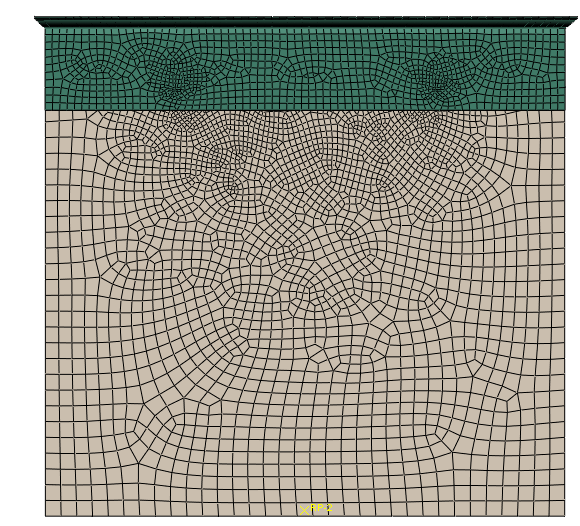
Figure 3: Mesh used when geometry is partitioned to describe screw locations.

Approach 2: Defining Fasteners on the Screw Locations

In a second approach, we will use the same mesh as in the previous example, but in this case mesh independent fasteners will connect the panel to the frame instead of ties.

The locations of the fasteners must be specified via reference points, nodes or attachment points. In this case reference points are defined by selecting the center of the screw in the geometry. When needing to define a number of connection points along a line, the “create attachment points along direction” option can be used to avoid specifying each point individually.

The “Create fasteners” options allows you to define fasteners. In this case the ‘point-based’ approach is used. The reference points corresponding to the fastener locations are selected. In this case two fastener definitions are made, one for the screws on the top and one for the screws on the bottom of the panel. In each case, the corresponding reference points are selected.

In the ‘domain’ tab of the ‘edit fasteners’ dialog box, the target surfaces need to be specified. There is a ‘whole model’ option, where Abaqus locates the surfaces itself. This cannot be used for coincident surfaces, as is the case in this example. Therefore, we use the ‘fasten specified surfaces by proximity’ option. The surfaces to be tied are specified, in this case a surface for the frame (top or bottom contact region) and one for the panel (top or bottom contact region).

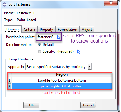
Figure 4: Specifying the fastener domain.

In the ‘property’ tab, the behavior of the fastener is specified. It is possible to use a connector section. This allows complex behavior, including non-linear and damage behavior. In this case we will keep things simple and use a rigid mpc connection. The physical radius of the fastener is specified as well. In this case we provide a value that corresponds to the size of the partitioned region.

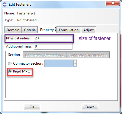
Figure 5: Specifying fastener properties.

Approach 3: Using Fasteners on a Coarse Mesh

In approach 2, the mesh was partitioned to separate the regions corresponding to the screws. This is not required in order to be able to define fasteners. In a third approach, these partitions are removed. A regular mesh is used, with elements that are larger than those around the screw location in the previous approach (Figure 6).

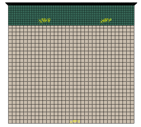
Figure 6: Mesh used when not including partitions to define the regions corresponding to the screws.

The number of elements is 6932 in this case, compared to 16409 (more than twice times as much) in the previous example.

Fasteners are defined as previously. This includes the physical radius specified. However, Abaqus also calculates a default radius of influence. If the user-specified radius of influence is smaller than the computed default radius of influence, the user-specified value will be overridden. In any case each region of influence will contain a minimum of three nodes. Given the mesh size, the region of influence will be larger than the value specified, to meet these requirements.

Approach 4: Tie Constraint on Complete Contact Surfaces

In the last approach tested, the complete surfaces in contact were tied to each other. In this case the same mesh as used in approach 3 was used. The location of the screws is not taken into account.

Results

When looking at the stress and strain results (Figure 7 and Figure 8), the results of both models with the screw geometry included in the mesh (approach 1 and 2) are very similar. Apparently using a tie or using fasteners does not have a big impact on the results in this case. Approach 3, with fasteners defined on a regular mesh that did not include partitions for the screws, shows a localization effect in the screw region, as is observed with approach 1 and 2, but the effect is more spread out. Because the effective radius of influence was larger in this analysis than in the other analysis, this is not unexpected. The fourth approach, with ties throughout the contact region, does not show a localization effect, as expected.

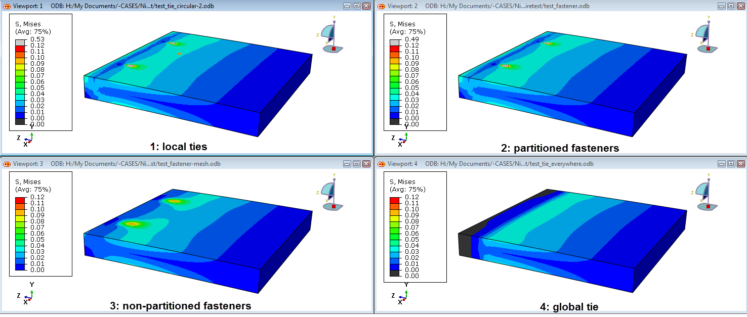
Figure 7: Von Mises stress using each of the 4 approaches.

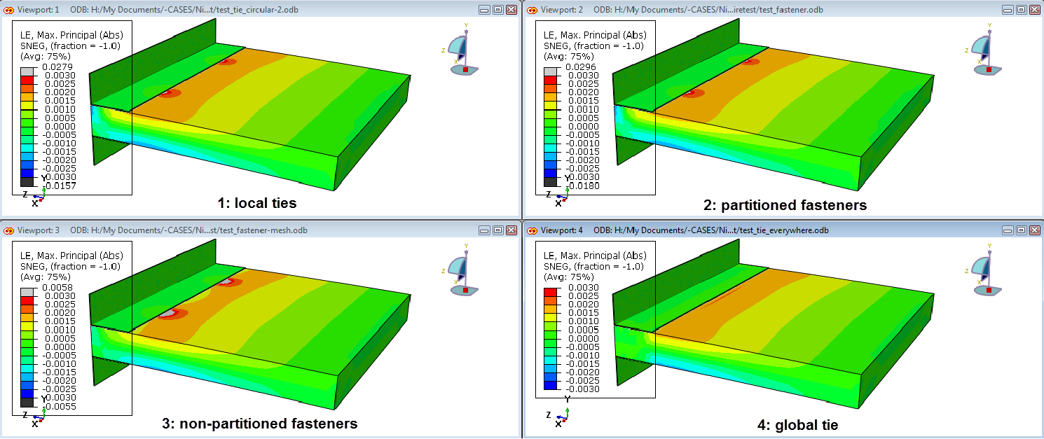
Figure 8: Maximal principal logarithmic strain using each of the 4 approaches.

When looking at displacement results (Figure 9) we see that the results for approach 1 and 2 overlap. With approach 3, the displacement is smaller, indicating the model behaves stiffer. This can be explained by the larger region that is included in the connection in this case. With approach 4, the fully tied contact regions, the displacement is even smaller, indicating an even stiffer response. This was expected.

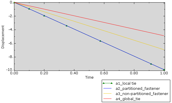
Figure 9: Displacement for the point at which the load is applied using each of the 4 approaches. The results for approach 1 and 2 overlap.

Furthermore, run times are given in the table below:

(These are according to the message file. No effort was taken to make the computational load due to other factors on the system constant, so these values are only meant to provide a rough estimate.)

This shows that the run time of the coarser models (3 and 4) is clearly less than that of the finer models. The difference between the local tie and the fastener model with the same mesh is small.

Conclusion

The approach using fasteners is easy to set-up, because it does not require partitioning of the mesh. This also makes meshing easier. The fastening points need to be defined, which takes some effort, but this is limited, especially when the linear patterning option to create attachment points can be used.

In this case, the connecting surfaces needed to be defined. This was done separately for the top and bottom of the panel. With a tie definition, all surface segments can be collected in a single master and a single slave surface, which is relatively fast.

All in all, defining non-partitioned fasteners is expected to be faster than defining partitioned ties in general.

It is possible to obtain results with a coarser mesh using the non-partitioned fastener approach compared to the partitioned ties. The result is less accurate, but it may be sufficient in some cases and the running time is much shorter. Refining the mesh in the non-partitioned approach is expected to reduce the difference between the non-partitioned and the partitioned approach (while of course increasing the running time).

Because the influence radius of the fastener is increased beyond the distance specified for coarse meshes, this approach is more mesh sensitive.

Using a non-partitioned fastener approach seems valuable when the level of detail and accuracy required is not too high, while running time and ease of setting up is important. It may also be useful as a first approach to get an idea of running times and how a model behaves, before going to more detailed modeling.