Why It Is Good to Understand What Your Fe Solver Is Doing (and How You Can Become More Knowledgeable As Well!)

While doing support we get all kinds of questions. I want to share one with you in this blog, because it was insightful for me, and I hope it will be insightful for others as well.

The Issue

The customer observes a different stress for different element types and wants to know why this happened.

The Model

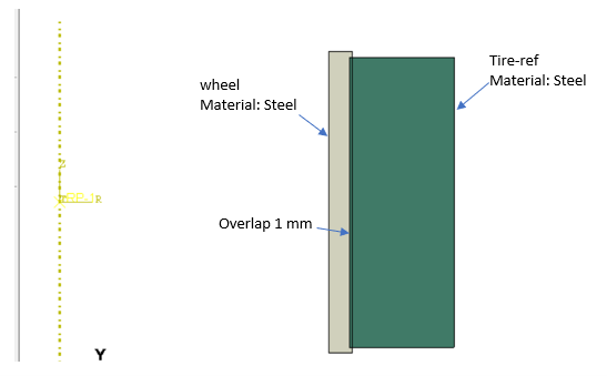
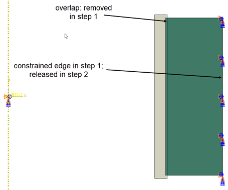
The model is fairly simple: it is axisymmetric with two parts. They initially overlap. During the first step, the overlap is removed using an interference fit while the edge furthest from the axis is fully constrained. During the second step this constraint is removed.

Figure 1: Model.

Investigation - Postprocessing

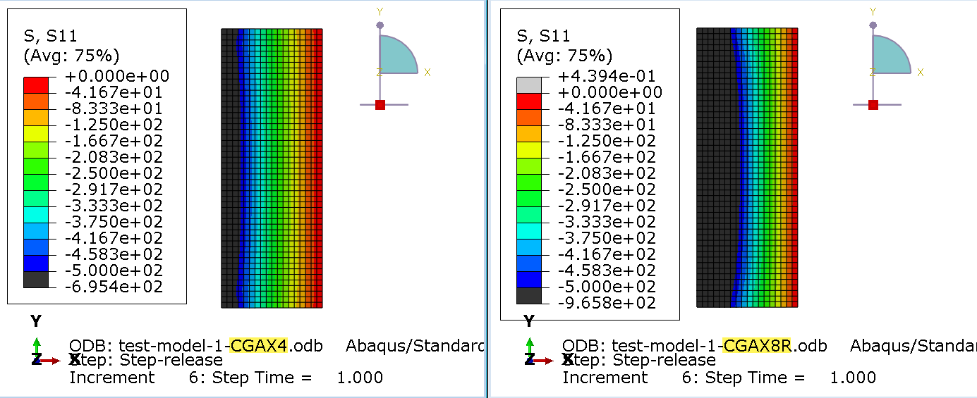
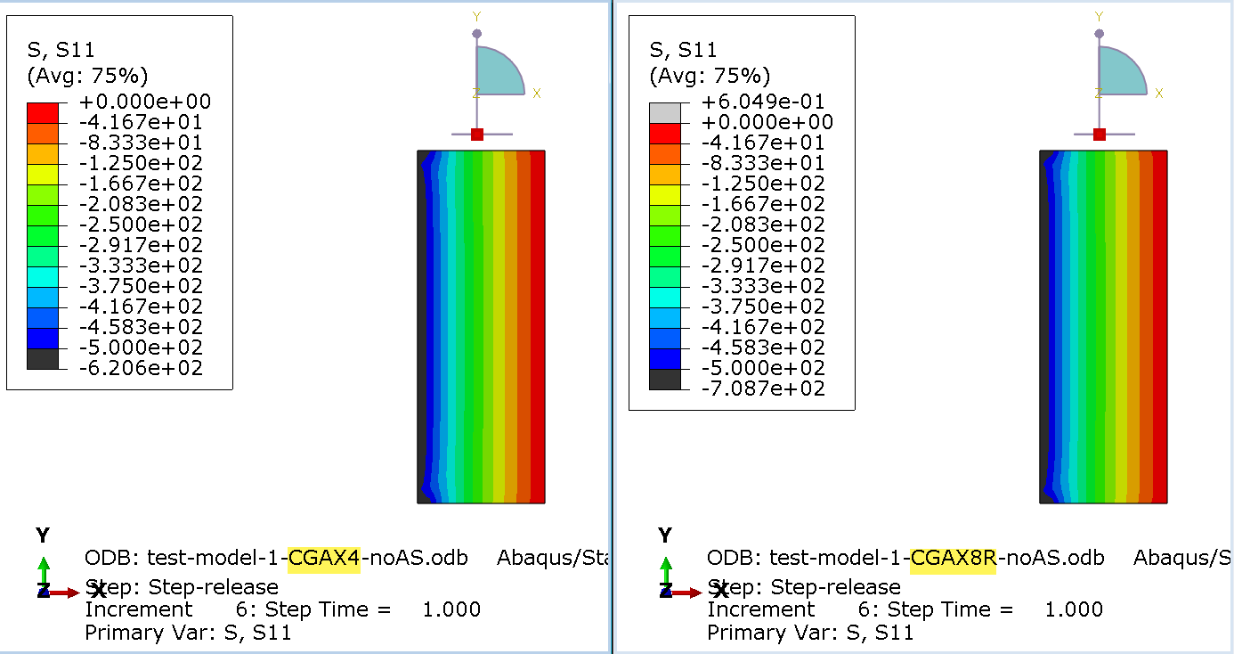
So what can be going on here? I first wanted to ensure the issue was not due to postprocessing. The average stress was calculated by summing the values at all integration points and dividing that by (the number of elements x the number of integration points per element). I decided to focus on CGAX4 and CGAX8R since the have the biggest difference and the same number of integrations points. I made various contour plots to avoid the postprocessing. Consistent with the average values provided, the stress in the analysis using CGAX8R elements is consistently more negative values than the stress in the analysis using CQAX4 elements. Around half of the model is below -500 for CGAX8R, only a quarter for CQAX4 (Figure 2). This means this is not due to postprocessing, but something seen in the results.

Figure 2: S11 with CQAX4 elements (left) and CQAX8R (right). The stress is consistently more negative (more towards the blue side of the spectrum for CGAX8R elements compared to CGAX4.

Investigation – Mesh Refinement

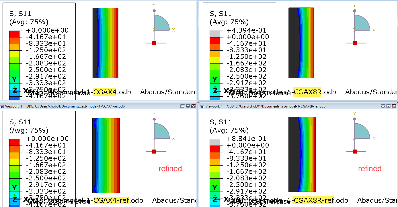
If it is not related to postprocessing, then what is it? It could be related to the element formulation. All elements should show the same behaviour if a fine enough mesh is used. I therefore refined the mesh in different models, to see whether the results were getting closer.

Figure 3: S11 for both element types for original mesh (top) and refined mesh (bottom). The same legend scale is used in all cases.

Unfortunately, the results did not get closer. If anything changed, the difference became larger.

Investigation – Model Set-up

So let’s take a good look at the model definition and what we expect to happen. (Perhaps I should have started with that, but better late than never). What is happening here?

Figure 4: overview of model, showing boundary conditions.

First, the overlap is removed while constraining the outer edge. Then the boundary condition is removed. So what do we expect to happen? Initially, the tire is compressed between the rim and the boundary condition. When the boundary condition is removed, it will no be completely stress free, because it is axisymmetric, but the stress level in the model should be low. It is essentially loaded and then unloaded.

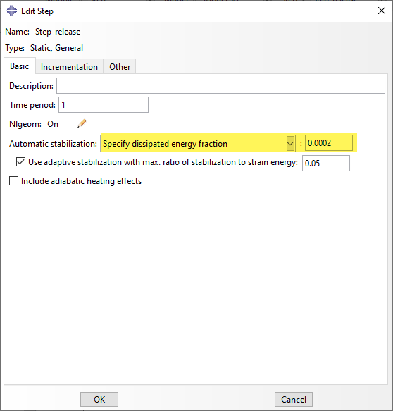
In the definition of both steps, automatic stabilization is switched on, using default settings.

Figure 5: Automatic stabilization.

Automatic stabilization is a very nice option, intended to improve convergence for models with local instabilities. Damping is applied: a force proportional to the nodal velocity resisting the motion is added. This stabilizes rigid body modes, sudden energy release due to loss of contact, etc. It can be used when going from one stabile state to another stable state, with unstable states in between, that aren’t of interest.

Since this is a non-physical effect, it should not dominate the solution. It can be challenging to determine a sensible damping parameter directly, which is why usually the dissipated energy fraction is defined. In this case Abaqus determines the damping factor based on the initial strain energy, in such a way that the dissipated energy for a given increment with characteristics similar to the first increment is a specified fraction of the extrapolated strain energy.

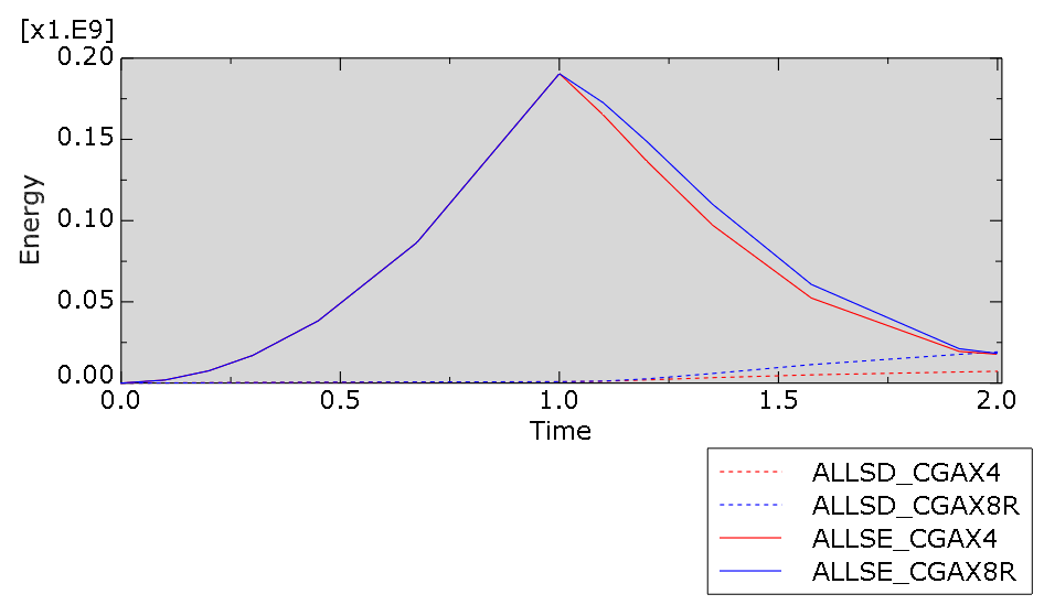
We can plot ALLSD (dissipated energy due to stabilization) and ALLSE (strain energy), to check whether ALLSD is indeed small (Figure 6).

Figure 6: Dissipation energy (dashed lines) and strain energy (solid lines) for model with CGAX4 elements (red) and model with CGAX8R elements (blue).

This shows that ALLSD is not small compared to ALLSE: it is approximately equal (CGAX8R) or around half (CGAX4). It also shows that the dissipation is different in both models. It is therefore likely the cause of the discrepancy in results.

Confirmation of Hypotheses

To test whether automatic stabilization causes the different S11 at the end of step 2 the analysis is run without automatic stabilization in either step. This convergences, indicating automatic stabilization was not necessary.

Figure 7: Results without automatic stabilization. The results now match.

Explanation

So, why does automatic stabilization have such a big impact in this case?

To my knowledge, Abaqus determines the damping factor assuming the loading will linearly increase during the step. This is what happens in step 1, and in this case ALLSD is small, as intended. For step 2, however, the loading reduces. If the damping factor is based on an expected linear increase, then the dissipation is small compared to a much larger stain energy. If the loading in fact reduces, then the estimated damping factor is much too large and the dissipation dominates the solution, as is observed here.

Recommended Usage

Automatic stabilization should be used with care. Start by running the analysis without it and do not include it unless it is needed. If you do use it, check the stabilization energy. Ensure the first increment is representative for the rest of the step and pay special attention to unloading steps.

Conclusion

Getting an Abaqus job to converge can be tricky, especially if contact is involved. Abaqus offers functionality to improve convergence, such as automatic stabilization. It is important to understand what an option does and when it can or cannot be applied if you want to have trustworthy results.